Tutorials

In this tutorial we will process and post-process receiver function data for station MMPY. This will include calculating receiver functions using all default arguments, re-calculating the receiver functions for different processing arguments, plotting them, and post-processing them using the H-k stacking technique and applying the harmonic decomposition method.

0. Creating the `StDb` Database

All the scripts provided require a StDb database containing station information and metadata. Let’s first create this database for station MMPY and send the prompt to a logfile

$ query_fdsn_stdb -N NY -S MMPY MMPY > logfile

To check the station info for MMPY, use the program ls_stdb:

$ ls_stdb MMPY.pkl
Listing Station Pickle: MMPY.pkl
NY.MMPY
--------------------------------------------------------------------------
1) NY.MMPY
     Station: NY MMPY
      Alternate Networks: None
      Channel: HH ;  Location: --
      Lon, Lat, Elev:  62.61892, -131.26247,   0.000
      StartTime: 2013-07-01 00:00:00
      EndTime:   2020-10-26 15:28:46
      Status:    partial
      Polarity: 1
      Azimuth Correction: 0.000000

1. Download and process receiver functions

You can see above that the station MMPY has been in operation between July 2013 and October 2020 (Note: the date at which the tutorial was written). In theory, we could run the main script to perform the automatic processing of the seismic data (rfpy_calc) using for example:

$ rfpy_calc MMPY.pkl

However, in this example we would be looking at over seven years of data, which is much more than we need for this tutorial. Note also that we didn’t specify a station key, since there is only one station in the data base. By default, rfpy_calc would process data for all teleseismic P-waves from earthquakes with magnitudes between 6 and 9 and with epicentral distances between 30 and 90 degrees that occurred between July 2013 and October 2020. The default component alignment is ZRT and the default deconvolution method is the wiener filter.

Let’s run an example where we want to limit the time range, include earthquakes with magnitude down to 5.5, change the component alignment and the deconvolution method:

$ rfpy_calc --minmag=5.5 --start=2017-05-01 --end=2017-10-31 --align=LQT --method=multitaper

An example log printed on the terminal will look like:

|===============================================|
|===============================================|
|                       MMPY                    |
|===============================================|
|===============================================|
|  Station: NY.MMPY                             |
|      Channel: HH; Locations: --               |
|      Lon: -131.26; Lat:  62.62                |
|      Start time: 2013-07-01 00:00:00          |
|      End time:   2020-10-26 15:28:46          |
|-----------------------------------------------|
| Searching Possible events:                    |
|   Start: 2017-05-01 00:00:00                  |
|   End:   2017-10-31 00:00:00                  |
|   Mag:   5.5 - 9.0                            |
| ...                                           |
|  Found   179 possible events                  |
|===============================================|

**************************************************
* #1 (5/179):  20170503_044713 NY.MMPY
* Requesting Waveforms:
*    Startime: 2017-05-03 04:56:33
*    Endtime:  2017-05-03 05:01:33
*     MMPY.HH - ZNE:
*          HH[ZNE].-- - Checking Network
*              - ZNE Data Downloaded
* Start times are not all close to true start:
*   HHE 2017-05-03T04:56:33.230000Z 2017-05-03T05:01:34.220000Z
*   HHN 2017-05-03T04:56:33.230000Z 2017-05-03T05:01:34.220000Z
*   HHZ 2017-05-03T04:56:33.230000Z 2017-05-03T05:01:34.220000Z
*   True start: 2017-05-03T04:56:33.229590Z
* -> Shifting traces to true start
* Waveforms Retrieved...
**************************************************

...

And so on until all data have been downloaded and processed. At that point you should have a new folder named P_DATA/NY.MMPY containing all event folders, each of them containing the meta data, station data, raw data, and receiver function data:

$ ls -R * | head

MMPY.csv
MMPY.pkl
P_DATA

./P_DATA:
NY.MMPY

./P_DATA/NY.MMPY:
20170503_044713
20170509_015414

Once this step is done, you can still re-calculate the receiver functions using different processing options (see below). However, some parameters cannot be changed easily without re-downloading the raw data (e.g., length of processing window, sampling rate). If you want to change those parameters, run the previous command with -O to override anything that exists on disk.

Note that you can get more data by either specifying a new phase to analyze (e.g., --phase=PP), going to lower magnitudes (e.g., --minmag=5. --maxmag=5.5), by running the same line of command with those additional arguments.

2. Re-calculate with different options

If later on you decide you want to try a different deconvolution method, component alignment or maybe try some pre-filtering options, you can always simply use the rfpy_recalc script to do so.

Note

Re-calculating the receiver functions for different options will override any existing receiver function data. Be mindful of this when using this script.

This can be done by typing in the terminal:

$ rfpy_recalc --align=ZRT --method=wiener MMPY.pkl

3. Plot receiver functions by back-azimuth or slowness

Now that we have our data set of receiver functions, we can plot it! There are two types of plots: the Back-azimuth panels and the Slowness panels. In the first case the receiver functions are sorted by back-azimuth and all slowness information is lost (i.e., averaged out). In the same case it is the opposite and the receiver fuuntions are sorted by slowness and all back-azimuth information is lost. When plotting, you can decide whether to include all data, or set some quality control thresholds based on 1) SNR of vertical component, 2) CC value of predicted and observed radial components, and 3) outliers. If you don’t specify any thresholding, by default the script rfpy_plot will use all data in the plots. You also want to set corner frequencies for filterig, otherwise it will be difficult to see anything. Typically you would choose a bandwidth that encompasses the dominant frequencies of teleseismic P waves (i.e., 0.05 to 1 Hz). Let’s examine the two types of plots with examples:

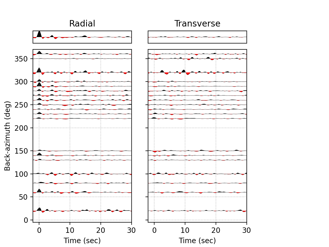
Back-azimuth panel

Below we make a plot of all P receiver functions, filtered between 0.05 and 0.5 Hz, using 36 back-azimuth bins. We plot the RFs from -2. to +30 seconds following the zero-lag (i.e., P-wave arrival) time, stack all traces to produce an averaged RF, and normalize all traces to that of the stacks.

$ rfpy_plot --no-outlier --bp=0.05,0.5 --nbaz=36 --normalize --trange=-2.,30. MMPY.pkl

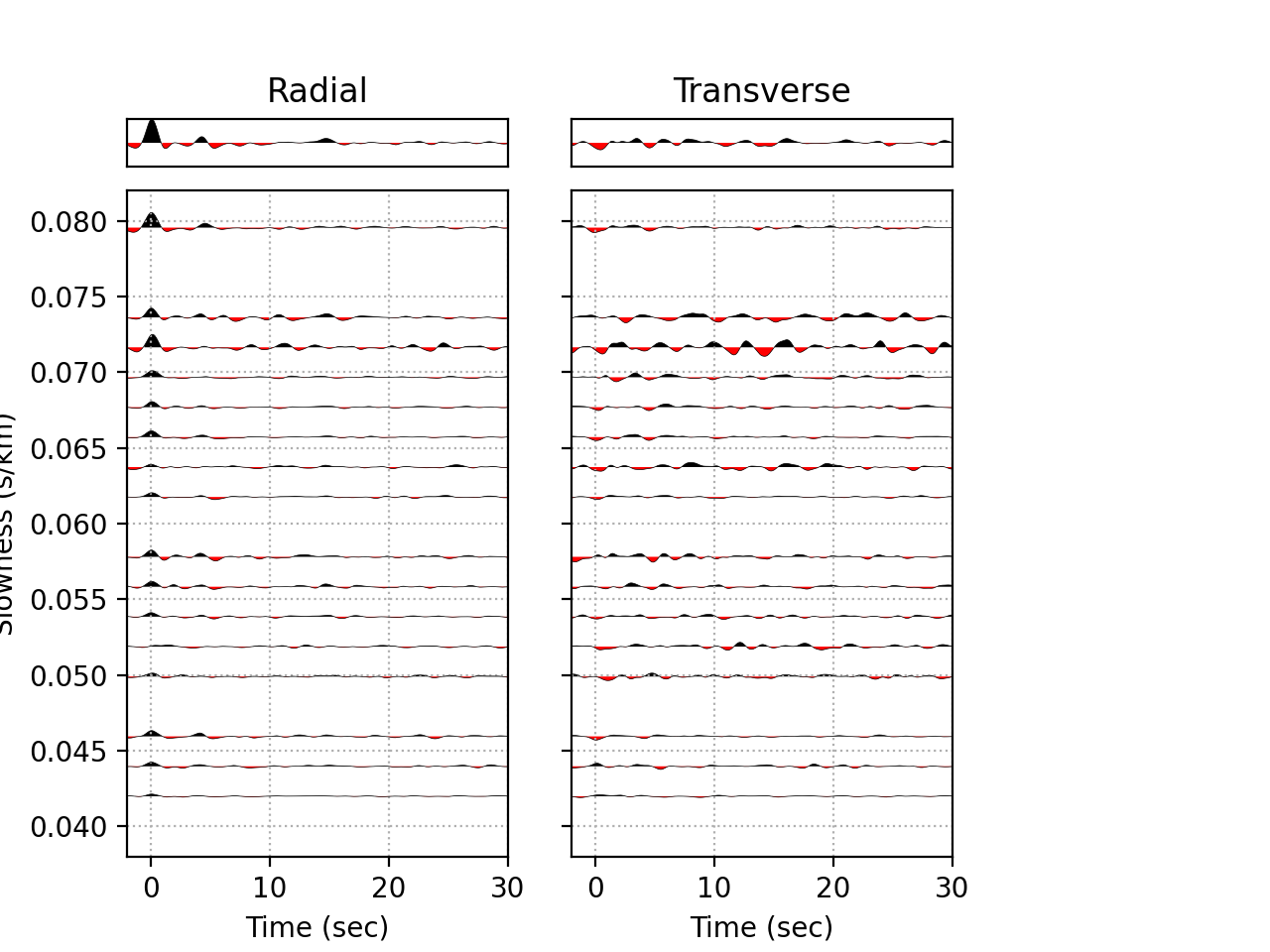
Slowness panel

Now let’s make a plot of all P receiver functions, this time sorted by slowness using 20 bins. Instead

$ rfpy_plot --no-outlier --bp=0.05,0.5 --nslow=20 --normalize --trange=-2.,30. MMPY.pkl

4. Post-processing

4a. Moho depth and Vp/Vs from `H-k` stacking

With these receiver functions, we can easily estimate Moho depth and crustal Vp/Vs using the simple H-k stacking method. There are several options to choose from. Let’s examine the default options.

$ rfpy_hk MMPY.pkl

By default the script will use all available receiver functions (no thresholding), bin them using 36 back-azimuth and 40 slowness bins, and stack them using H and k intervals of 0.5 and 0.02, respectively, with bounds of [20., 50] and [1.56, 2.1], respectively for H and k search. The weights for the Ps, Pps and Pss phases is [0.5, 2., -1] and the final H-k stack will be the weighted sum of all 3 phases. The default crustal Vp value to use in calculating the phase arrival time is 6.0 km/s. Finally, after computing the stacks, nothing is done and the code stops. To produce a plot and save the results to disk requires adding processing arguments.

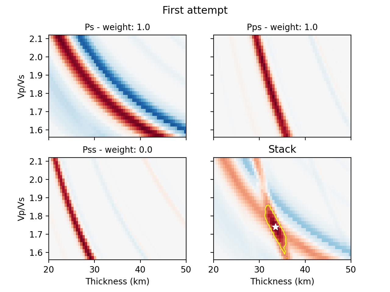
As an example, let’s remove outliers, using 20 slowness bins (instead of 40 to speed things up), change the weights to [1., 1., 0], change the Vp to 5.5 km/s, save the H-k object and make a plot with some title:

$ rfpy_hk --no-outlier --nslow=20 --weights=1.,1.,0. --vp=5.5 --save --plot --title='First attempt' MMPY.pkl

#########################################
#        __                 _     _     #
#  _ __ / _|_ __  _   _    | |__ | | __ #
# | '__| |_| '_ \| | | |   | '_ \| |/ / #
# | |  |  _| |_) | |_| |   | | | |   <  #
# |_|  |_| | .__/ \__, |___|_| |_|_|\_\ #
#          |_|    |___/_____|           #
#                                       #
#########################################

Path to HK_DATA/NY.MMPY doesn`t exist - creating it


|===============================================|
|===============================================|
|                       MMPY                    |
|===============================================|
|===============================================|
|  Station: NY.MMPY                             |
|      Channel: HH; Locations: --               |
|      Lon: -131.26; Lat:  62.62                |
|      Start time: 2013-07-01 00:00:00          |
|      End time:   2020-10-26 15:28:46          |
|-----------------------------------------------|

Number of radial RF data: 90


Number of radial RF bins: 16

Computing: [#####..........] 24/61

Once computing is done (when it reaches 61/61), the script will produce the following figure:

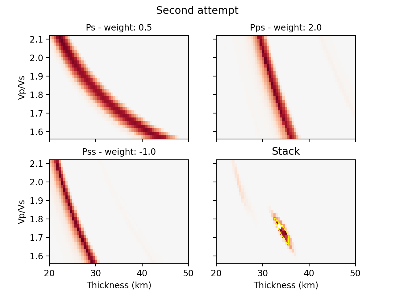
Alternatively, we can compute the stacks using the product of all phase stacks, which gets rid of the subjective choice of weights. Let’s re-do the prevous example with a number of changes: 1) use a copy of the RFs to use for the reverberations (Pps and Pss), 2) bandpass filter those at lower high-frequency corner, and 3) select the ‘product’ method.

$ rfpy_hk --no-outlier --nslow=20 --vp=5.5 --copy --bp-copy=0.05,0.35 --type=product --save --plot --title='Second attempt' MMPY.pkl

The new figure is slightly different (there is no negative amplitude) but produces much cleaner H and k estimates. Note that the labeled weights above each panel correspond to the default values but are not used in the final stack.

Finally, could also perform H-k stacking using a known orientation (strike and dip angles) of a dipping interface using additional arguments.

4b. Harmonic decomposition

Receiver functions are often characterized by significant amplitude variations as a function of back-azimuth of the incoming teleseismic wave. The variations are observed on both radial and transverse components, with a 90-degree shift (in back-azimuth) between the two components. The harmonic decomposition method exploits these variations by decomposing the amplitude (at each time interval) into a set of harmonic components that describe the periodicity in receiver function amplitudes. See Audet (2015) for details on the methodology.

The default arguments will perform the decomposition over all receiver functin data at a fixed azimuth of 0 degrees (i.e., North), such that the second and third components represent 1-theta variations oriented in the N-S and E-W directions, calculated over the first 10 seconds of the receiver function data:

$ rfpy_harmonics MMPY.pkl

This command simply runs the decomposition algorithm but does not return anything, unless you specify the --save and/or the --plot command. Instead of the default 0-degree azimuth, you can set the azimuth at which you wish to perform the decomposition by setting the --azim= argument. It is also possible to estimate the azimuth at which one of the harmonic components will be minimized (typically the second or third term), in order to reveal the dominant orientation of the receiver function amplitudes. This is accomplished using the --find-azim argument. Finally, you can also set the range of lag times over which to calculate the decomposition (--trange=; default is from 0 to 10 seconds) and perform the decomposition for a selected date range (--start= and --end=). Other QC control arguments are similar to previous scripts.

Let’s perform the decomposition by estimating the dominant azimuth using a time range of 2 to 10 seconds (to avoid the large zero-lag pulse):

Note

Warning!! This command is particularly slow, especially for large data sets.

$ rfpy_harmonics --no-outlier --find-azim --trange=2.,10. MMPY.pkl

################################################################################
#        __                 _                                      _           #
#  _ __ / _|_ __  _   _    | |__   __ _ _ __ _ __ ___   ___  _ __ (_) ___ ___  #
# | '__| |_| '_ \| | | |   | '_ \ / _` | '__| '_ ` _ \ / _ \| '_ \| |/ __/ __| #
# | |  |  _| |_) | |_| |   | | | | (_| | |  | | | | | | (_) | | | | | (__\__ \ #
# |_|  |_| | .__/ \__, |___|_| |_|\__,_|_|  |_| |_| |_|\___/|_| |_|_|\___|___/ #
#          |_|    |___/_____|                                                  #
#                                                                              #
################################################################################



|===============================================|
|===============================================|
|                       MMPY                    |
|===============================================|
|===============================================|
|  Station: NY.MMPY                             |
|      Channel: HH; Locations: --               |
|      Lon: -131.26; Lat:  62.62                |
|      Start time: 2013-07-01 00:00:00          |
|      End time:   2020-10-26 15:28:46          |
|-----------------------------------------------|

Decomposing receiver functions into baz harmonics
Optimal azimuth for trange between 2.0 and 10.0 seconds is: 178.0

Now that we have the estimated azimuth, we can re-calculate the decomposition using --azim= and plot them over the first 20 seconds.

$ rfpy_harmonics --no-outlier --azim=178. --trange=2.,10., --plot --ymax=20. --title="Decomposition at azimuth 178 degrees" MMPY.pkl

This command will produce the following figure:

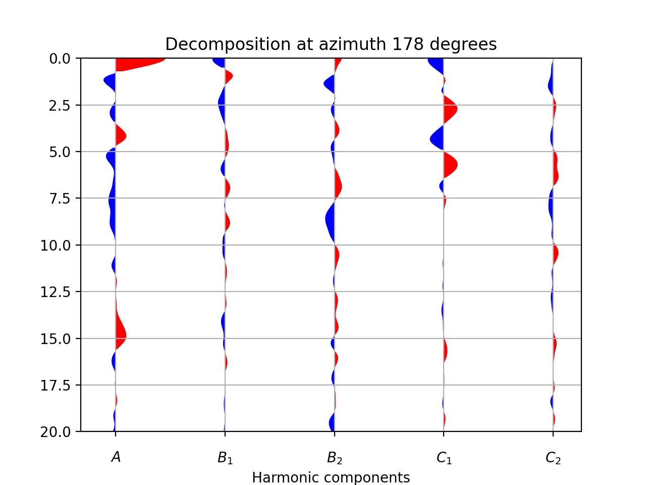
The first component (A) shows the amplitudes that do not vary with back-azimuth (i.e., the ‘constant’ term), with the main Ps and Pps Moho-related pulses at 3. and 15. seconds. The second component (B1) has been minimized between 2. and 10. seconds and does not show any significant signal. The third component (B2) shows the amplitudes at the optimal azimuth of 178 degrees, with a pair of positive-negative pulses at around 7 and 8 seconds. Finally, the fourth component (C1) shows some high-amplitude signals between 2.5 and 6 seconds, which correspond to hexagonal anisotropy with a horizontal axis of symmetry.