Licence

Copyright 2019 Pascal Audet

Permission is hereby granted, free of charge, to any person obtaining a copy of this software and associated documentation files (the “Software”), to deal in the Software without restriction, including without limitation the rights to use, copy, modify, merge, publish, distribute, sublicense, and/or sell copies of the Software, and to permit persons to whom the Software is furnished to do so, subject to the following conditions:

The above copyright notice and this permission notice shall be included in all copies or substantial portions of the Software.

THE SOFTWARE IS PROVIDED “AS IS”, WITHOUT WARRANTY OF ANY KIND, EXPRESS OR IMPLIED, INCLUDING BUT NOT LIMITED TO THE WARRANTIES OF MERCHANTABILITY, FITNESS FOR A PARTICULAR PURPOSE AND NONINFRINGEMENT. IN NO EVENT SHALL THE AUTHORS OR COPYRIGHT HOLDERS BE LIABLE FOR ANY CLAIM, DAMAGES OR OTHER LIABILITY, WHETHER IN AN ACTION OF CONTRACT, TORT OR OTHERWISE, ARISING FROM, OUT OF OR IN CONNECTION WITH THE SOFTWARE OR THE USE OR OTHER DEALINGS IN THE SOFTWARE.

Installation

Dependencies

The current version has been tested using Python > 3.6 Also, the following packages are required:

• stdb

• spectrum

• cartopy

Other required packages (e.g., obspy) will be automatically installed by stdb.

Conda environment

We recommend creating a custom conda environment where RfPy can be installed along with some of its dependencies.

conda create -n rfpy python=3.9 obspy cartopy -c conda-forge

Activate the newly created environment:

conda activate rfpy

Install remaining dependencies using pip inside the rfpy environment:

pip install stdb
pip install spectrum

Installing from Pypi

pip install rfpy

Installing from source

• Clone the repository:

git clone https://github.com/paudetseis/RfPy.git
cd RfPy

• Install using pip:

pip install .

Basic Usage

Calculating Receiver Functions

The basic class of RfPy is RFData, which contains attributes and methods for the calculation of single-station, teleseismic P-wave receiver functions from three-component seismograms. A RFData object contains three main attributes: a StDb object with station information, a Meta object containing event meta data, and a Stream object containing the unrotated 3-component seismograms. Additional processing attributes are added as the analysis proceeds. The sequence of initialization and addition of attributes is important, as described in the documentation below.

Note that, at the end of the process, the RFData object will further contain a Stream object as an additional attribute, containing the receiver function data.

Note

A RFData object is meant to facilitate processing of single-station and single-event P-wave receiver functions. For processing multiple event-station pairs, an equal number of RFData objects need to be created. See the accompanying Scripts for details.

Initialization

A RFData object is initialized with an StDb object, e.g. consider such an object sta:

>>> from rfpy import RFData
>>> rfdata = RFData(sta)

Once the object is initialized, the first step is to add an obspy.core.event.Event` object. For example, given such an object ev:

>>> rfdata.add_event(ev)

Now that the event has been added, the RFData object has determined whether or not it is suitable for receiver function analysis (i.e., if the event is within a suitable epicentral distance range), which is available as a new meta attribute:

>>> rfdata.meta.accept
True

Note

Alternatively, the add_event() (or add_data()) method can be used with the argument returned=True to return the accept attribute directly.

>>> rfdata.add_event(ev, returned=True)
True

If the accept attribute is True, continue with the analysis by adding raw three-component data. There are two methods to perform this step. If the data are available in memory (e.g., in a Stream object stream), one can use the add_data() method directly:

>>> rfdata.add_data(stream)

Warning

Do not simply add a Stream object as an attribute data to the RFData object (e.g., rfdata.data = stream). Instead use this method, as it checks whether or not the data are suitable for receiver function analysis.

Otherwise, one can use the method download_data() to obtain the three-component data from an FDSN Client:

>>> rfdata.download_data(client)

The accept attribute will be updated with the availability of the data attribute, i.e. if no data is available, the accept attribute will be set to False. The methods to add data can also be used with the argument returned=True to report whether or not the data are available.

Receiver function processing

Now that we have complete meta data and raw seismogram data, we can use methods to rotate and/or calculate the signal-to-noise ratio. The rotation flag is set in the rfdata.meta.align attribute, which by default is 'ZRT'. This means that 'ZNE' data will be rotated to 'ZRT' before deconvolution, automatically. However, we can set a different alignment (e.g., 'LQT' or 'PVH') and perform the rotation prior to deconvolution. Once rotation is performed, however, the initial 'ZNE' data is no longer available and further rotation cannot be performed:

>>> rfdata.rotate()
>>> rfdata.meta.rotated
True
>>> rfdata.meta.align
'ZRT'
>>> rfdata.rotate(align='PVH')
...
Exception: Data have been rotated already - aborting

The SNR is calculated based on the align attribute, on the first component (e.g., either 'Z', 'L' or 'P'). Therefore, this method is typically carried out following the rotate method:

>>> rfdata.calc_snr()
>>> type(rfdata.meta.snr)
float

Finally, the last step is to perform the deconvolution using the method deconvolve(), which stores the receiver function data as a new attribute rf, which is a three-component Stream object:

>>> rfdata.deconvolve()

Although no plotting method is provided for the RFData object, the rf attribute is a Stream object that can be plotted using the plot() method (e.g., rfdata.rf.plot()).

Following receiver function deconvolution, all the information is stored in the attributes of the object. Ultimately, a method is available to convert the RFData object to a Stream object with new attributes:

>>> rfstream = rfdata.to_stream()

Demo example

To look at a concrete example for station MMPY, consider the demo data provided with the package and process them using all default values:

>>> from rfpy import RFData
>>> rfdata = RFData('demo')
Uploading demo station data - station NY.MMPY

Check out its attributes (initialization only stores the sta attribute)

>>> rfdata.__dict__
{'sta': {'station': 'MMPY',
  'network': 'NY',
  'altnet': [],
  'channel': 'HH',
  'location': ['--'],
  'latitude': 62.618919,
  'longitude': -131.262466,
  'elevation': 0.0,
  'startdate': 2013-07-01T00:00:00.000000Z,
  'enddate': 2599-12-31T23:59:59.000000Z,
  'polarity': 1.0,
  'azcorr': 0.0,
  'status': 'open'},
 'meta': None,
 'data': None}

Now import an event:

>>> rfdata.add_event('demo')
2014-06-30T19:55:33.710000Z | +28.391, +138.873 | 6.2 MW

Print the content of the object meta data

>>> rfdata.meta.__dict__
{'time': 2014-06-30T19:55:33.710000Z,
 'lon': 138.8727,
 'lat': 28.3906,
 'dep': 527.4,
 'mag': 6.2,
 'epi_dist': 7236.909875705126,
 'az': 30.556903955991746,
 'baz': 283.91831389584587,
 'gac': 65.08309411308255,
 'ttime': 588.38610458337996,
 'slow': 0.056707554238157355,
 'inc': 19.167277207756957,
 'phase': 'P',
 'accept': True,
 'vp': 6.0,
 'vs': 3.5,
 'align': 'ZRT',
 'rotated': False,
 'snr': None,
 'snrh': None,
 'cc': None}

Note

Once the event object is loaded, it is possible to edit the attributes of meta, although we recommend only editing vp, vs or align, and avoid editing any of the station-event attributes

>>> rfdata.meta.vp = 5.5
>>> rfdata.meta.vs = 3.3
>>> rfdata.meta.vp, rfdata.meta.vs
(5.5, 3.3)
>>> rfdata.meta.align = 'LQT'
>>> rfdata.meta.align
'LQT'

Now add data to the object:

>>> rfdata.add_data('demo')
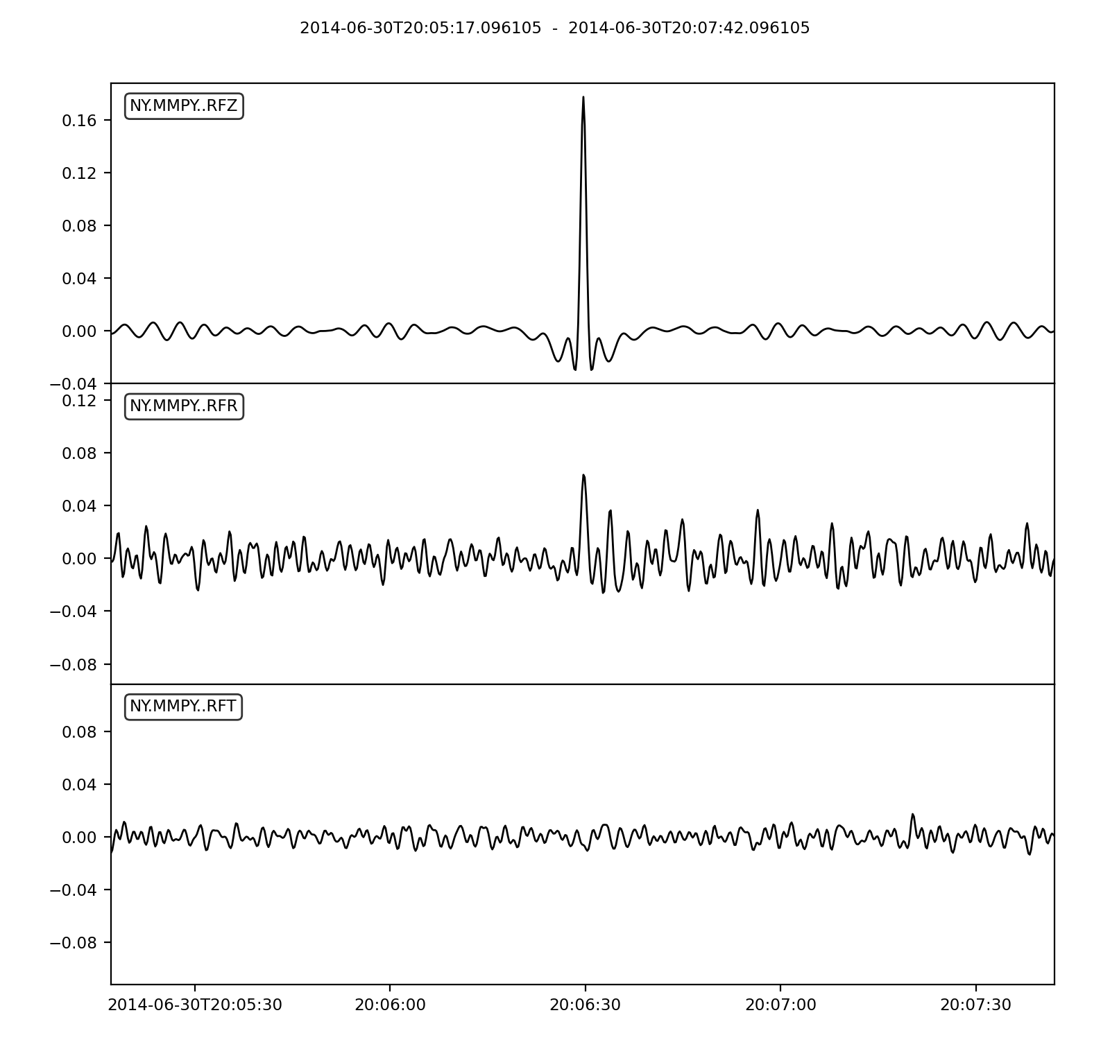
3 Trace(s) in Stream:
NY.MMPY..HHZ | 2014-06-30T20:02:52.096105Z - 2014-06-30T20:07:51.896105Z | 5.0 Hz, 1500 samples
NY.MMPY..HHN | 2014-06-30T20:02:52.096105Z - 2014-06-30T20:07:51.896105Z | 5.0 Hz, 1500 samples
NY.MMPY..HHE | 2014-06-30T20:02:52.096105Z - 2014-06-30T20:07:51.896105Z | 5.0 Hz, 1500 samples

Perform receiver function deconvolution using default values:

>>> rfdata.deconvolve()
Warning: Data have not been rotated yet - rotating now
Warning: SNR has not been calculated - calculating now using default

>>> rfdata.rf
3 Trace(s) in Stream:
NY.MMPY..RFZ | 2014-06-30T20:05:17.096105Z - 2014-06-30T20:07:42.096105Z | 5.0 Hz, 726 samples
NY.MMPY..RFR | 2014-06-30T20:05:17.096105Z - 2014-06-30T20:07:42.096105Z | 5.0 Hz, 726 samples
NY.MMPY..RFT | 2014-06-30T20:05:17.096105Z - 2014-06-30T20:07:42.096105Z | 5.0 Hz, 726 samples

>>> rfstream = rfdata.to_stream()
>>> rfstream
3 Trace(s) in Stream:
NY.MMPY..RFZ | 2014-06-30T20:05:17.096105Z - 2014-06-30T20:07:42.096105Z | 5.0 Hz, 726 samples
NY.MMPY..RFR | 2014-06-30T20:05:17.096105Z - 2014-06-30T20:07:42.096105Z | 5.0 Hz, 726 samples
NY.MMPY..RFT | 2014-06-30T20:05:17.096105Z - 2014-06-30T20:07:42.096105Z | 5.0 Hz, 726 samples

Check out new stats in traces

>>> rfstream[0].stats.snr
18.271607454697513
>>> rfstream[0].stats.slow
0.056707554238157355
>>> rfstream[0].stats.baz
283.91831389584587
>>> rfstream[0].stats.is_rf
True

Plot filtered and trimmed rfstream

>>> rfstream.filter('bandpass', freqmin=0.05, freqmax=0.5, corners=2, zerophase=True)
>>> rfstream.plot()

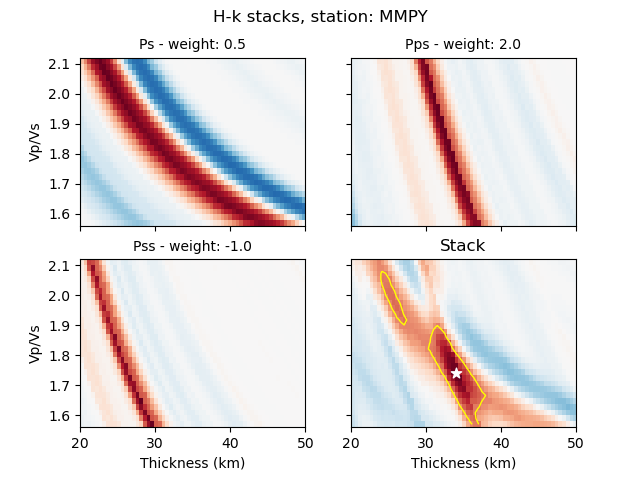
Post-Processing: H-k stacking

The class HkStack contains attributes and methods to calculate thickness (H) and Vp/Vs ratio (k) of the crust (in reality, H refers to Moho depth, and k is Vp/Vs of the medium from the surface to H) based on moveout times of direct Ps and reverberated Pps and Pss phases from radial-component receiver functions. The individual phase stacks are obtained from the median weighted by the phase of individual signals. Methods are available to combine the phase stacks into a weighted sum or a product.

Initialization

A HkStack object is initialized with a Stream object containing radial receiver function data. The Stream is built by adding (or appending) radial receiver functions obtained from valid RFData objects using the to_stream() method.

>>> from rfpy import HkStack
>>> hkstack = HkStack(rfstream)

The rfstream typically requires minimal pre-processing, such as bandpass filtering to enhance the converted and reverberated phases. For example:

>>> rfstream.filter('bandpass', freqmin=0.05, freqmax=0.75, corners=2, zerophase=True)
>>> hkstack = HkStack(rfstream)

Note

It is also possible to use two rfstream objects during initialization of the HkStack object - one for the direct conversion (i.e., 'ps' phase), and the second one for the reverberated phases (i.e., 'pps', 'pss'). The second rfstream should therefore be a copy of the first one, but perhaps filtered uding different frequency corners:

>>> rfstream2 = rfstream.copy()
>>> rfstream2.filter('bandpass', freqmin=0.05, freqmax=0.35, corners=2, zerophase=True)
>>> hkstack = HkStack(rfstream, rfstream2)

To speed things up during processing (and to avoid redundant stacking), it is possible to use one of the binning() functions, alghouth not the bin_all() function, e.g.,

>>> from rfpy.binning import bin
>>> rfstream_binned = rfstream.bin(typ='slow', nbin=21)
>>> hkstack = HkStack(rfstream_binned)

H-k processing

Once the HkStack object is initialized with the rfstream, a findividual phase stacks can be calculated automatically using the default settings:

>>> hkstack.stack()

The only parameter to set is the P-wave velocity of the crust - if not set, the default value of 6.0 km/s is used (available as the attribute hkstack.vp). To change the search bounds for the phase stacks, we can edit the attributes of the HkStack object prior to calling the method stack():

>>> hkstack.hbound = [15., 40.]
>>> hkstack.dh = 1.5
>>> hkstack.kbound = [1.6, 2.0]
>>> hkstack.dk = 0.01
>>> hkstack.stack(vp=5.5)

Warning

Setting small values for hkstack.dh and hkstack.dk will slow down the processing significantly, but produce much cleaner and more precise stacks.

In the presence of a dipping Moho interface, it is possible to use the method stack_dip(), with the additional strike and dip arguments. If not specified, the code will use the default values stored as attributes of the HkStack object:

>>> hkstack.stack_dip(strike=215., dip=25., vp=5.5)

Once the phase stacks are calculated and stored as attributes of the object, we can call the method average() to combine the phase stacks into a single, final stack. By default the final stack is a simple weighted sum of the individual phase stacks, using weights defined as object attributes:

>>> hkstack.weights
[0.5, 2., -1.]
>>> hkstack.average()

To produce a final stack that consists of the product of the positive parts of individual phase stacks (to enhance normal-polarity Moho arrivals and ignore un-modelled negative polarity signals), use the typ='product' argument:

>>> hkstack.average(typ='product')

The estimates of H and k are determined from the maximum value in the final stack as attributes hkstack.h0 and hkstack.k0. The method will also call the error() method to calculate the errors and error contour around the solution.

The individual and final stacks can be plotted by calling the method plot():

>>> hkstack.plot()

Demo example

Initialize object with demo data for station MMPY:

>>> from rfpy import HkStack
>>> hkstack = HkStack('demo')
Uploading demo data - station NY.MMPY

>>> # Check content of object
>>> hkstack.__dict__
{'rfV1': 198 Trace(s) in Stream:

NY.MMPY..RFR | 2014-06-29T17:27:39.906888Z - 2014-06-29T17:28:52.306888Z | 5.0 Hz, 363 samples
...
(196 other traces)
...
NY.MMPY..RFR | 2014-07-15T16:51:48.381573Z - 2014-07-15T16:53:00.781573Z | 5.0 Hz, 363 samples

[Use "print(Stream.__str__(extended=True))" to print all Traces],
 'rfV2': None,
 'strike': None,
 'dip': None,
 'vp': 6.0,
 'kbound': [1.56, 2.1],
 'dk': 0.02,
 'hbound': [20.0, 50.0],
 'dh': 0.5,
 'weights': [0.5, 2.0, -1.0],
 'phases': ['ps', 'pps', 'pss']}

These receiver functions have been obtained by adding RFData objects as streams to an Stream object, without other processing. Note that they are aligned in the 'PVH' coordinate system, as specified in the channel name (i.e., 'RFV' for the radial component). To prepare them for stacking, we can bin the receiver functions into back-azimuth and slowness bins (in the presence of a dipping interface), or simply slowness bins (for horizontal interfaces):

>>> from rfpy import binning
>>> rfV_binned = binning.bin(hkstack.rfV1, typ='slow', nbin=21)[0]
>>> hkstack.rfV1 = rfV_binned

it is straightforward to directly filter the Stream object, and perhaps also add a copy of the stream with a different frequency corner as another attribute rfV2, as suggested above:

>>> hkstack.rfV2 =  hkstack.rfV1.copy()
>>> hkstack.rfV1.filter('bandpass', freqmin=0.05, freqmax=0.5, corners=2, zerophase=True)
>>> hkstack.rfV2.filter('bandpass', freqmin=0.05, freqmax=0.35, corners=2, zerophase=True)

Now simply process the hkstack object using the default values to obtain H and k estimates

>>> hkstack.stack()
Computing: [###############] 61/61

>>> hkstack.average()

The final estimates are available as attributes

>>> hkstack.h0
34.0
>>> hkstack.err_h0
3.5
>>> hkstack.k0
1.74
>>> hkstack.err_k0
0.13

Plot the stacks with error contours

>>> hkstack.plot()

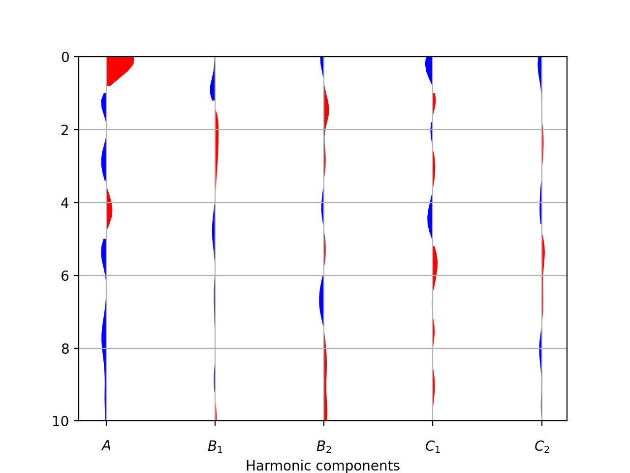
Post-Processing: Harmonic Decomposition

The class Harmonics contains attributes and methods to calculate the first five harmonic components of radial and transverse component receiver function data from a singular value decomposition. The harmonic decomposition can be performed at a fixed azimuth (i.e., along some known dominant strike direction in the subsurface), or alternatively the decomposition can be optimized to search for the dominant azimuth that maximizes the energy on one of the components. This direction can be interpreted as the strike of a dipping interface or can be related to anisotropic axes.

Initialization

a Harmonics object is initialized with both radial and transverse component receiver function Stream objects. The Stream objects are built by adding (or appending) radial and transverse receiver functions obtained from valid RFData objects using the to_stream() method.

>>> from rfpy import Harmonics
>>> harmonics = Harmonics(rfRstream, rfTstream)

Note

The rfRstream and rfTstream typically require minimal pre-processing, such as bandpass filtering to enhance the converted and reverberated phases. For example:

>>> rfRstream.filter('bandpass', freqmin=0.05, freqmax=0.75, corners=2, zerophase=True)
>>> rfTstream.filter('bandpass', freqmin=0.05, freqmax=0.75, corners=2, zerophase=True)
>>> harmonics = Harmonics(rfRstream, rfTstream)

Warning

The radial and transverse components should not be mixed, and should contain purely radial and purely transverse components (i.e. no mixing of components). Furthermore, the Stream objects should have equal length and the same ordering.

Harmonic decomposition

Once the Harmonics object is initialized, processing is done by typing:

>>> harmonics.dcomp_fix_azim()

Or, alternatively,

>>> harmonics.dcomp_find_azim()

In either case the harmonic components are available as an attribute of type Stream (harmonics.hstream) and, if available, the azimuth of the dominant direction (harmonics.azim).

Note

When using the method rfpy.harmonics.dcomp_find_azim(), it is possible to specify a range of values over which to perform the search using the arguments xmin and xmax, where x refers to the independent variable (i.e., time or depth, if the streams have been converted from time to depth a priori).

Once the harmonic decomposition is performed, the components can be plotted using the method plot()

>>> harmonics.plot()

Forward modeling

If the hstream attribute is available, it is possible to forward model receiver functions for a range of back-azimuth values, or just a single value. In case the back-azimuths are not specified, the method will use the range of values available in the original radial and transverse component receiver function data.

>>> harmonics.forward()

The new predicted radial and transverse component receiver functions are available as attributes of type Stream (harmonics.forwardR and harmonics.forwardT)

Demo example

Initialize object with demo data for station MMPY:

>>> from rfpy import Harmonics
>>> harmonics = Harmonics('demo')
Uploading demo data - station NY.MMPY

>>> # Check content of object
>>> harmonics.__dict__
{'radialRF': 198 Trace(s) in Stream:

NY.MMPY..RFR | 2014-06-29T17:27:39.906888Z - 2014-06-29T17:30:04.906888Z | 5.0 Hz, 726 samples
...
(196 other traces)
...
NY.MMPY..RFR | 2014-07-15T16:51:48.381573Z - 2014-07-15T16:54:13.381573Z | 5.0 Hz, 726 samples

[Use "print(Stream.__str__(extended=True))" to print all Traces],
 'transvRF': 198 Trace(s) in Stream:

NY.MMPY..RFT | 2014-06-29T17:27:39.906888Z - 2014-06-29T17:30:04.906888Z | 5.0 Hz, 726 samples
...
(196 other traces)
...
NY.MMPY..RFT | 2014-07-15T16:51:48.381573Z - 2014-07-15T16:54:13.381573Z | 5.0 Hz, 726 samples

[Use "print(Stream.__str__(extended=True))" to print all Traces],
 'azim': 0,
 'xmin': 0.0,
 'xmax': 10.0}

As with the HkStack object, these receiver functions have been obtained by adding RFData objects as streams to an Stream object, without other processing. Note that they are aligned in the 'PVH' coordinate system, as specified in the channel name (i.e., 'RFV' and 'RFH'). To prepare them for harmonic decomposition, we can bin the receiver functions into back-azimuth and slowness bins :

>>> from rfpy import binning
>>> str_binned = binning.bin_baz_slow(harmonics.radialRF, harmonics.transvRF)
>>> harmonics.radialRF = str_binned[0]
>>> harmonics.transvRF = str_binned[1]

It is straightforward to directly filter the Stream object, and perhaps also add a copy of the stream with a different frequency corner as another attribute rfV2, as suggested above:

>>> harmonics.radialRF.filter('bandpass', freqmin=0.05, freqmax=0.5, corners=2, zerophase=True)
>>> harmonics.transvRF.filter('bandpass', freqmin=0.05, freqmax=0.5, corners=2, zerophase=True)

Now simply perform harmonic decomposition

>>> harmonics.dcomp_fix_azim()
Decomposing receiver functions into baz harmonics for azimuth =  0

Plot them

>>> harmonics.plot(ymax=10.)