Example 3: Invert a Receiver Function
In this example we are going to load receiver functions that have been
created from seismograms recorded at station Hyderabad, India, from 3
earthquakes that occurred in the Philippines. The source station
configuration is identical to the one in example 1. We are going to use
pyraysum to generate receiver function, as in example 2. This
example explores the provisions of pyraysum for time optimized
execution. We are going to directly invoke the Fortran routine
run_bare() from the fraysum module with python convenience
functions from the prs module. The inversion will be carried out by
the dual_annealing() function from scipy.optimize. The filtering
and spectral division that is required to create receiver functions from
the synthetic seismograms is carried out using numpy array methods.
finally, we will plot the results with matplotlib.
from pyraysum import prs, frs
from fraysum import run_bare
import numpy as np
import scipy.optimize as spo
import matplotlib.pyplot as mp
Definition of the Forward Computation
We predict waveforms inside a function predictRF() that accepts
Model, Geometry, and RC objects, which completely define the
synthetic seismograms to be computed. Only the fthickn and fvs
attributes of the Model will be varied when trying different
parameter combinations. The post-processing is determined by the
bandpass filter corner frequencies freqs and the boolean time window
mask ist (“is time”). Post processing is performed on the
numpy.ndarray variable rfarray. Two post-processing functions
are provided. filtered_rf_array divides the SV- and SH-spectra by
the P-spectra (i.e., computes a receiver function) and filters the data,
whereas filtered_array returns the filtered SV and SH data.
def predictRF(model, geometry, rc, freqs, rfarray, ist, rf=True):

    # Compute synthetic seismograms
    traces = run_bare(
        model.fthickn,
        model.frho,
        model.fvp,
        model.fvs,
        model.fflag,
        model.fani,
        model.ftrend,
        model.fplunge,
        model.fstrike,
        model.fdip,
        model.nlay,
        *geometry.parameters,
        *rc.parameters
    )

    if rf:
        # Perfrom spectral division and filtering
        frs.filtered_rf_array(
            traces, rfarray, geometry.ntr, rc.npts, rc.dt, freqs[0], freqs[1]
        )
    else:
        # Perfrom filtering only
        frs.filtered_array(
            traces, rfarray, geometry.ntr, rc.npts, rc.dt, freqs[0], freqs[1]
        )

    # Window traces and flatten array
    # This creates alternating radial and transverse RFs for all traces:
    # R[0] - T[0] - R[1] - T[1] ...
    prediction = rfarray[:, :, ist].reshape(-1)

    return prediction
Definition of the Misfit Function
Here, we define the misfit function that dual_annealing will
minimize. The misfit function requires a model vector theta as first
argument. We define the first element of the model vector to be the
crustal thickness and the second one the P-to-S-wave velocity ratio.
\(V_P/V_S\) gets projected to the S-wave velocity assuming a
constant P-wave velocity. After that, we define the misfit cost
between the predicted and observed receiver functions (pred and
obs, respectively) as 1. minus the cross correlation coefficient. A
status message is printed so the user can follow the inversion process.
def misfit(theta, model, geometry, rc, freqs, rfarray, ist, obs):

    # Set parameters to model object
    model.fthickn[0] = theta[0]
    model.fvs[0] = model.fvp[0] / theta[1]

    # predict receiver functions
    pred = predictRF(model, geometry, rc, freqs, rfarray, ist)

    # Calculate cross correlation cost function
    cost = 1.0 - np.corrcoef(obs, pred)[0][1]

    msg = "h ={: 5.0f}, vpvs ={: 5.3f}, cc ={: 5.3f}".format(
        theta[0], theta[1], 1. - cost
    )

    print(msg)

    return cost
Plotting Function for Data vs. Model Prediction
This plot function allows us to compare the observed and predicted data vectors:
def plot(obs, pred):
    fig, ax = mp.subplots(nrows=1, ncols=1)
    fig.suptitle("Observed and modeled data vector")

    imid = len(obs)//2
    cc = np.corrcoef(obs, pred)[0][1]
    title = "cc = {:.3f}".format(cc)

    ax.plot(obs, color="dimgray", linewidth=2, label="observed")
    ax.plot(pred, color="crimson", linewidth=1, label="modeled")
    ax.text(imid, min(pred), 'Radial ', ha='right')
    ax.text(imid, min(pred), ' Transverse', ha='left')
    ax.axvline(imid, ls=':')
    ax.legend(title=title)
    ax.spines[["top", "left", "right"]].set_visible(False)
    ax.set_yticks([])
    ax.set_xlabel("Sample")
Inversion Workflow
Recording Geometry
Now it is time to run the workflow. We define the back-azimuth and slowness of seismic rays arriving at Hyderabad from the Philippines. The time window should span the interval between 0 and 25 seconds after the arrival of the direct P-wave. Data should be bandpassed filtered between periods of 20 and 2 seconds.
if __name__ == "__main__":
    baz = 90
    slow = 0.06

    twind = (0, 25)  # seconds time window
    freqs = (1 / 20, 1 / 2)  # Hz bandpass filter
Loading a Receiver Function
We load the radial and transverse receiver functions from file. The
receiver function has been created from 3 high-quality earthquake
recordings from the Philippines. Note that rfr and rft here need
to be structured such that the arrival of the direct P-wave is located
in the middle of the array. In other words, the acausal part (earlier
than direct P) must be as long as the causal part (later than direct P).
In this way, the definition of the time window mask ist is such that
it can be reused for post-processing of the synthetic receiver
functions. The windowed receiver function are concatenated to yield the
data vector.
# Load saved stream
time, rfr, rft = np.loadtxt("../data/rf_hyb.dat", unpack=True)
ist = (time > twind[0]) & (time < twind[1])

observed = np.concatenate((rfr[ist], rft[ist]))
Setup of Starting Model and Run Control Parameters
We set up the starting subsurface velocity model using Saul et al. (2000), as well as the recording geometry.
thickn = [30000, 0]
rho = [2800, 3600]
vp = [6400, 8100]
vs = [3600, 4600]

model = prs.Model(thickn, rho, vp, vs)
geometry = prs.Geometry(baz, slow)
We choose the RC parameters so that they match the processing of the
receiver functions. In the present case, the receiver functions are
rotated to the P-SV-SH ray coordinate system (rot=2), and the
sampling interval (dt) and number of samples (npts) are set to
match the input. The align=1 option (together with shift=None,
which is the default) ensures that the direct P wave is located at the
first sample. mults=3 is required to pre-set the list of phases to
be computed. This is the recommended option for all time-sensitive
applications, as mults=2 computes many multiples, many of which
might not be used at all.
rc = prs.Control(
    verbose=False,
    rot=2,
    dt=time[1] - time[0],
    npts=len(rfr),
    align=1,
    mults=3,
)
Definition of a Custom Phaselist
The phaselist is defined as a list of phase descriptors, which can be
read from a previous forward calculation (e.g. example 1). Each ray
segment is described by a number-letter pair, where the number is the
layer index and the letter the phase descriptor, where uppercase
indicates upgoing rays and lowercase downgoing rays. See the
rc.set_phaselist documentation for details.
This phaselist restricts the phases to be computed to:
direct P (P)
P-to-S converted (PS)
P reflected at the surface to downgoing S, reflected at Moho to S (PpP)
P reflected at the surface to downgoing P, reflected at Moho to S (PpS)
P reflected at the surface to downgoing S, reflected at Moho to P (PsP)
You can try the effect of incorporating PsS by adding "1P0P0s0S"
to the phaselist. The equivalent=True keyword implicitly adds such
equivalent phases.
Note: PpS and PsP phases arrive at the same time, but only phases that end in S are directly visible on the receiver function. Phases ending in P end up on the P polarized trace of the synthetic seismogram, where they become part of the denominator of spectral division when computing the receiver function.)
rc.set_phaselist(["1P0P", "1P0S", "1P0P0p0P", "1P0P0p0S", "1P0P0s0P"], equivalent=True)
Faster Array-Based Postprocessing
Swift post processing of the synthetic receiver function is done on the
rfarray using numpy array methods, which is initialized here. It has
shape (geometry.ntr, 2, rc.npts).
rfarray = frs.make_array(geometry, rc)
A First Look at the Observed and Predicted Data Vectors
Let’s see how well the starting model predicts the data. See what
changes if you set rf=False, in which case no spectral division is
performed and the model prediction is the synthetic seismogram. This
expedites the computation, but is less exact.
predicted = predictRF(model, geometry, rc, freqs, rfarray, ist, rf=True)
plot(observed, predicted)
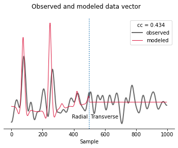
The first half of the data vector is the radial component and the second half is the transverse component of the receiver function. In this example, without dip or anisotropy, energy only gets converted to the radial, not the transverse component. The first positive wiggle is PS, the second one PpS. Note the slight mis-alignment between observation (gray) and prediction (red). The smaller wiggles that arrive later result from the deconvolution of PpP.
Inverse Modeling with Scipy’s Optimize Module
We now define the search bounds for dual annealing. This definition prescribes that the first element of the model vector is the thickness of layer 0 and is searched in an interval of \(\pm 5000\) m, and its second element is the \(V_P/V_S\) ratio of layer 0*, searched in an interval of \(\pm\) 0.1.
bounds = [
    (model[0, "thickn"] - 5000, model[0, "thickn"] + 5000),
    (model[0, "vpvs"] - 0.1, model[0, "vpvs"] + 0.1),
]
Now we are ready to perform the inversion using scipy’s dual
annealing
function. It seeks a minimum in the misfit function defined above.
The call is in principle interchangeable with other global search
methods from the optimization
module.
result = spo.dual_annealing(
    misfit,
    bounds,
    args=(model, geometry, rc, freqs, rfarray, ist, observed),
    maxiter=20,
    seed=42,
)
h = 28745, vpvs = 1.868, cc = 0.408
h = 27107, vpvs = 1.690, cc =-0.028
h = 32605, vpvs = 1.826, cc = 0.542
h = 31991, vpvs = 1.826, cc = 0.645
h = 31991, vpvs = 1.805, cc = 0.697
h = 31991, vpvs = 1.805, cc = 0.697
h = 31991, vpvs = 1.805, cc = 0.697
h = 31991, vpvs = 1.805, cc = 0.697
h = 27506, vpvs = 1.877, cc =-0.611
h = 29815, vpvs = 1.865, cc = 0.622
h = 30922, vpvs = 1.865, cc = 0.673
h = 30922, vpvs = 1.818, cc = 0.695
h = 28651, vpvs = 1.841, cc = 0.307
h = 33587, vpvs = 1.873, cc = 0.110
h = 31375, vpvs = 1.873, cc = 0.598
h = 31375, vpvs = 1.877, cc = 0.598
h = 25540, vpvs = 1.762, cc =-0.109
h = 27033, vpvs = 1.678, cc =-0.002
h = 34752, vpvs = 1.678, cc = 0.528
h = 34752, vpvs = 1.699, cc = 0.482
h = 28105, vpvs = 1.706, cc = 0.023
h = 27870, vpvs = 1.750, cc =-0.346
h = 34876, vpvs = 1.750, cc = 0.351
h = 34876, vpvs = 1.809, cc = 0.144
h = 33399, vpvs = 1.817, cc = 0.400
h = 32429, vpvs = 1.826, cc = 0.563
h = 33830, vpvs = 1.826, cc = 0.246
h = 33830, vpvs = 1.720, cc = 0.603
h = 25188, vpvs = 1.778, cc =-0.134
h = 29661, vpvs = 1.691, cc = 0.034
h = 33416, vpvs = 1.691, cc = 0.654
h = 33416, vpvs = 1.744, cc = 0.611
h = 33839, vpvs = 1.825, cc = 0.246
h = 33327, vpvs = 1.694, cc = 0.660
h = 25421, vpvs = 1.694, cc = 0.024
h = 25421, vpvs = 1.874, cc =-0.542
h = 31451, vpvs = 1.679, cc = 0.352
h = 31523, vpvs = 1.763, cc = 0.682
h = 34688, vpvs = 1.763, cc = 0.339
h = 34688, vpvs = 1.685, cc = 0.528
h = 32610, vpvs = 1.855, cc = 0.406
h = 33846, vpvs = 1.751, cc = 0.520
h = 34880, vpvs = 1.751, cc = 0.351
h = 34880, vpvs = 1.738, cc = 0.377
h = 29890, vpvs = 1.861, cc = 0.627
h = 29687, vpvs = 1.760, cc = 0.282
h = 26578, vpvs = 1.760, cc =-0.208
h = 26578, vpvs = 1.730, cc =-0.102
h = 28745, vpvs = 1.707, cc = 0.007
h = 31883, vpvs = 1.754, cc = 0.699
h = 25874, vpvs = 1.754, cc =-0.137
h = 25874, vpvs = 1.772, cc =-0.167
h = 31883, vpvs = 1.754, cc = 0.699
h = 31883, vpvs = 1.754, cc = 0.699
h = 31883, vpvs = 1.754, cc = 0.699
h = 30617, vpvs = 1.829, cc = 0.683
h = 34402, vpvs = 1.849, cc = 0.072
h = 31076, vpvs = 1.849, cc = 0.686
h = 31076, vpvs = 1.765, cc = 0.612
h = 25822, vpvs = 1.847, cc =-0.442
h = 34603, vpvs = 1.721, cc = 0.466
h = 29529, vpvs = 1.721, cc = 0.102
h = 34603, vpvs = 1.740, cc = 0.421
h = 26306, vpvs = 1.680, cc = 0.011
h = 27198, vpvs = 1.705, cc =-0.090
h = 30551, vpvs = 1.705, cc = 0.250
h = 30551, vpvs = 1.829, cc = 0.669
h = 31185, vpvs = 1.686, cc = 0.301
h = 27166, vpvs = 1.848, cc =-0.560
h = 29608, vpvs = 1.848, cc = 0.540
h = 29608, vpvs = 1.766, cc = 0.279
h = 34714, vpvs = 1.746, cc = 0.394
h = 27866, vpvs = 1.763, cc =-0.385
h = 27651, vpvs = 1.763, cc =-0.344
h = 27651, vpvs = 1.743, cc =-0.259
h = 31781, vpvs = 1.873, cc = 0.530
h = 28840, vpvs = 1.683, cc =-0.021
h = 32547, vpvs = 1.683, cc = 0.591
h = 32547, vpvs = 1.786, cc = 0.659
h = 30755, vpvs = 1.809, cc = 0.670
h = 29781, vpvs = 1.726, cc = 0.157
h = 25482, vpvs = 1.726, cc =-0.030
h = 25482, vpvs = 1.694, cc = 0.048
h = 34650, vpvs = 1.697, cc = 0.518
h = 28644, vpvs = 1.747, cc = 0.066
h = 34869, vpvs = 1.747, cc = 0.351
h = 34869, vpvs = 1.868, cc =-0.030
Results
Let’s have a look at the result
print(result)
    fun: 0.3012503891104201
message: ['Maximum number of iteration reached']
   nfev: 87
   nhev: 0
    nit: 20
   njev: 2
 status: 0
success: True
      x: array([3.18828982e+04, 1.75376118e+00])
And assign it to the model
model[0, "thickn"] = result.x[0]
model[0, "vpvs"] = result.x[1]

msg = "Result found with dual annealing"
print(msg)
print(model)
Result found with dual annealing
#  thickn     rho      vp      vs  flag aniso   trend plunge strike   dip
  31882.9  2800.0  6400.0  3649.3    1    0.0     0.0    0.0    0.0   0.0
      0.0  3600.0  8100.0  4600.0    1    0.0     0.0    0.0    0.0   0.0
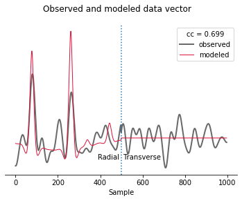
The optimal crustal thickness is closer to 32 km, as suggested by Saul et al. (2000), and the \(V_P/V_S\) ratio closer to 1.8. Note, however, that we only looked at one receiver function from one direction. We also did not make any attempt to estimate uncertainties on the solution.
Finally, we can look at how well the optimized model predicts the data.
predicted = predictRF(model, geometry, rc, freqs, rfarray, ist)
plot(observed, predicted)
Conclusion
In this example we looked into some basic functions that can be helpful
when using PyRaysum in parameter estimation problems. We defined a
function predictRF to predict a receiver function from a given input
model, as well as a misfit function whose scalar output should be
minimized through inverse modeling. We then plugged these functions into
SciPy’s optimize toolbox to estimate the thickness and S-wave
velocity of the cratonic crust in Hyderabad, India.
References
Saul, J., Kumar, M. R., & Sarkar, D. (2000). Lithospheric and upper mantle structure of the Indian Shield, from teleseismic receiver functions. Geophysical Research Letters, 27(16), 2357-2360. https://doi.org/10.1029/1999GL011128