Example 2: Reproducing Receiver Functions for Dipping and Anisotropic Subsurface Structure
In this example we generate P receiver functions for a model that includes either a dipping lower crustal layer or a lower-crustal anisotropic layer. These example reproduce the results of Figure 3 in Porter et al. (2011).
Start by importing the necessary packages:
from pyraysum import prs, Geometry, Model, Control
import numpy as np
Dipping Layers
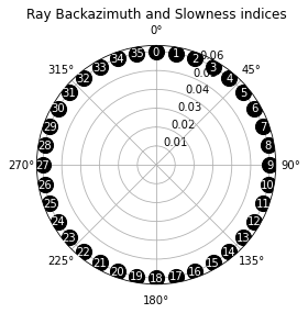
First we define the arrays of slowness and back-azimuth values of the
incident P wave to use as input in the simulation
baz = np.arange(0., 360., 10.)
slow = 0.06
geom = Geometry(baz, slow)
_ = geom.plot()
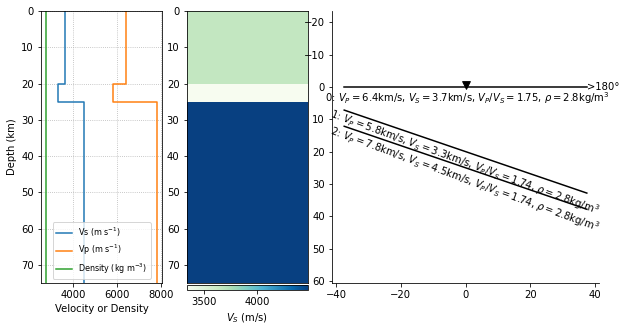
Next we define the model object. These values are found in the caption of Figure 3 in Porter et al. (2011). Note that \(V_S\) can be parameterized either directly or as \(V_P/V_S\), which is what we do here. Also note that values that are constant for all layers can be given as floats.
thickn = [20000, 5000, 0]
rho = 2800
vp = [6400, 5800, 7800]
vpvs = [1.75, 1.74, 1.74]
dip = [0, 20, 20]
strike = 90

model = Model(thickn, rho, vp, vpvs=vpvs, strike=strike, dip=dip)
model.plot()
print(model)
#  thickn     rho      vp      vs  flag aniso   trend plunge strike   dip
  20000.0  2800.0  6400.0  3657.1    1    0.0     0.0    0.0   90.0   0.0
   5000.0  2800.0  5800.0  3333.3    1    0.0     0.0    0.0   90.0  20.0
      0.0  2800.0  7800.0  4482.8    1    0.0     0.0    0.0   90.0  20.0
Now we specify the run-control parameters. Here we use the argument
rot=1 to produce seismograms aligned in the R-T-Z coordinate
system. The default value is rot=0, which produces seismograms
aligned in the N-E-Z coordinate system that should not be used
to calculate receiver functions. Furthermore, we are interested only in
the direct conversions, and therefore specify mults=0 to avoid
dealing with multiples. This is required to reproduce the published
examples, although it is good practice to keep all first-order multiples
to properly simulate all possible phase arrivals.
rc = Control(rot=1, mults=0, verbose=False, npts=1200, dt=0.0125)
Finally, let’s run the simulation. All book-keeping is handled internally.
result = prs.run(model, geom, rc)
The function returns a Result object whose attributes are the
Model, Geometry of incoming rays, a list of Streams as well
as all run-time arguments that are used by Raysum:
result.__dict__.keys()
dict_keys(['model', 'geometry', 'streams', 'rc', 'rfs'])
We can then use the method calculate_rfs() to calculate receiver
functions.
result.calculate_rfs()
The receiver functions are stored as an additional attribute of the
streamlist object, which is itself a list of Streams containing the
radial and transverse component RFs:
result.__dict__.keys()
dict_keys(['model', 'geometry', 'streams', 'rc', 'rfs'])
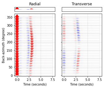
We can now filter and plot the results - we specify the key 'rfs' to
work on the receiver functions only.
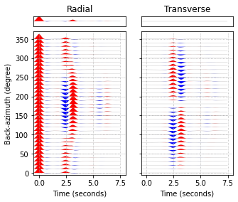
result.filter('rfs', 'lowpass', freq=1., zerophase=True, corners=2)
result.plot('rfs', tmin=-0.5, tmax=8.)
Anisotropic Layers
Now let’s reproduce the second case with the anisotropic lower crustal
layer. Here, the second layer (1 in python indexing) is not dipping,
but has a strong anisotropy of -20% (a negative value means a slow axis
of hexagonal symmetry). The anisotropy axis trends south
(trend = 180) and plunges 45 degree (plunge = 45). The P-wave
velocity is 6.2 km/s. We could define a new model as above. Another
possibility is to use use a short command string to change the existing
model.
Note that when we change the P-wave velocity and want to maintain a
constant \(V_P/V_S\) ratio, we must explicitly change vpvs by
changing vs. This is achieved using the 'pss' attribute
indicator below.
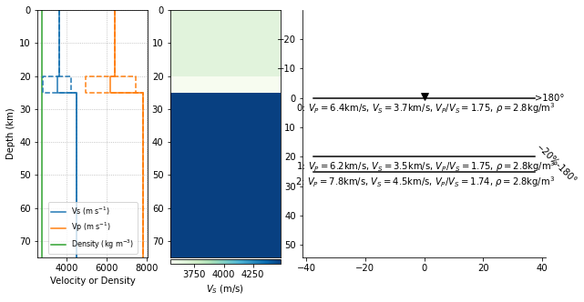
model.change('d1=0; d2=0; vp1=6.2; pss1=1.75; a1=-20; tr1=180; pl1=45;')
model.plot()
print(model)
Changed: dip[1] = 0.0
Changed: dip[2] = 0.0
Changed: vp[1] = 6200.0
Changed: vpvs[1] = 1.75
Changed: ani[1] = -20.0
Changed: trend[1] = 180.0
Changed: plunge[1] = 45.0
#  thickn     rho      vp      vs  flag aniso   trend plunge strike   dip
  20000.0  2800.0  6400.0  3657.1    1    0.0     0.0    0.0   90.0   0.0
   5000.0  2800.0  6200.0  3542.9    0  -20.0   180.0   45.0   90.0   0.0
      0.0  2800.0  7800.0  4482.8    1    0.0     0.0    0.0   90.0   0.0
Instead of two dipping interfaces, the model now has a thin anisotropic
layer at the base of the crust. We again compute synthetic seismograms
and use the rf argument to process the receiver functions as well.
result = prs.run(model, geom, rc, rf=True)

result.filter('rfs', 'lowpass', freq=1., zerophase=True, corners=2)
result.plot('rfs', tmin=-0.5, tmax=8.)
Understanding Fast and Slow S-Waves
To understand the different phases displayed, we can look at, e.g., the
receiver function at back-azimuth 150°. With a back-azimuthal spacing of
10°, the ray-index is 15. Let look into Geometry:
geom[15]
(150.0, 0.06, 0, 0)
Yes, the first value of the tuple is the back-azimuth, which is 150°.
The same index points into Result:
print(result[15])
(<obspy.core.stream.Stream object at 0x7f596a0616a0>, <obspy.core.stream.Stream object at 0x7f596a038700>)
The first element of the tuple are the synthetic seismograms, the second the receiver function:
print(result[15][0])
3 Trace(s) in Stream:
...SYR | 1970-01-01T00:00:00.000000Z - 1970-01-01T00:00:14.987500Z | 80.0 Hz, 1200 samples
...SYT | 1970-01-01T00:00:00.000000Z - 1970-01-01T00:00:14.987500Z | 80.0 Hz, 1200 samples
...SYZ | 1970-01-01T00:00:00.000000Z - 1970-01-01T00:00:14.987500Z | 80.0 Hz, 1200 samples
print(result[15][1])
2 Trace(s) in Stream:
...RFR | 1970-01-01T00:00:00.000000Z - 1970-01-01T00:00:14.987500Z | 80.0 Hz, 1200 samples
...RFT | 1970-01-01T00:00:00.000000Z - 1970-01-01T00:00:14.987500Z | 80.0 Hz, 1200 samples
We now look at how the individual phases are called and when they arrive.
print(result[15][0][0].stats.phase_descriptors)
print(result[15][0][0].stats.phase_times)
_ = result[15][0][0].plot()
['2P1P0P' '2P1P0S' '2P1S0S' '2P1T0S']
[0.01250004768371582 2.4625535011291504 3.0867090225219727
 3.174315929412842]
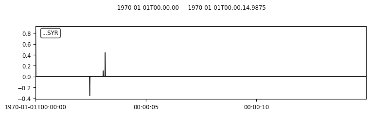
The commands above tell us that the negative wiggle arriving at 2.5 seconds is a P-to-S conversion at the bottom of layer 0 (i.e. the top of the anisotropic layer), whereas the positive wiggle at 3s consists of two S-waves arriving shortly after one another: The smaller wiggle is the P-to-S1 conversion at the bottom of layer 1 (the anisotropic layer), and the larger one is the P-to-S2 conversion at the same interface. (Note that the slow S-wave is denoted T, to avoid ambiguity with the layer indices.) Both phases travel as an S-wave (here again named T) in the topmost layer 0, but at different speeds.
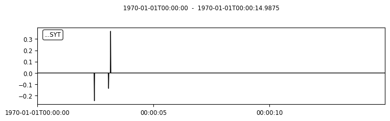
On the transverse component, the P-to-S1 conversion has a negative amplitude, while the P-to-S2 conversion has a larger, positive one.
print(result[15][0][1].stats.phase_descriptors)
print(result[15][0][1].stats.phase_times)

_ = result[15][0][1].plot()
['2P1P0T' '2P1S0T' '2P1T0T']
[2.4625535011291504 3.0867090225219727 3.174315929412842]
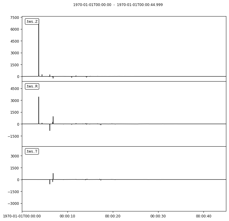
Validation against Telewavesim Data
As in the previous example, we would now like to compare these results with independently obtained results from Telewavesim. We’ll need NumPy to conveniently load our Telewavesim data from file, obspy to store them in a Stream object, and Matplotlib to make the comparison plot.
import obspy
import matplotlib.pyplot as mp
# Load telewavesim data
time, twr, twt, twz = np.loadtxt("../data/telewavesim_aniso_baz150-slow006.dat", unpack=True)

# Get time interval `dt` from data
dt = time[1] - time[0]

# Store into Stream, switch Z component polarity and set header
twsd = obspy.Stream()
for tr, channel in zip([twr, twt, twz], ["R", "T", "Z"]):
    header = {"delta": dt, "station": "tws", "channel": channel}
    trace = obspy.Trace(tr, header=header)
    twsd.append(trace)

# Make simple plot
_ = twsd.plot()
We’ll again filter both seismograms, as Telewavesim data does not provide a good infinite frequency approximation.
# Set frequency corners in Hz
fmin = 1./10.
fmax = 10
prsd = result.streams[15]
prsd.trim(endtime = prsd[0].stats.starttime+5)

# Demean and filter all data
for dat in [twsd, prsd]:
    dat.detrend("demean")
    dat.filter("bandpass", freqmin=fmin, freqmax=fmax, zerophase=True)
We also need to align the two different datasets to the direct P-wave and scale them to its amplitude on the vertical component.
# Index of the maximum amplitude on the vertical component of the data
imax = np.argmax(abs(prsd[2].data))

# Cycle through both synthetic data and process them equally
jmax = np.argmax(abs(twsd[2].data))  # maximum vertical amplitude
dt = prsd[2].times()[imax] - twsd[2].times()[jmax] # relative time shift of maximum
norm = prsd[2].data[imax] / twsd[2].data[jmax]  # relative amplitude of vertical maximum
for tr in twsd:
    tr.stats.starttime += dt  # align peaks
    tr.data *= norm  # normalize
    tr.trim(prsd[0].stats.starttime, prsd[0].stats.endtime)
For a good comparison, we use the plot function from the previous example:
def plot(data, model):

    lws = [4, 1]  # linewidths ...
    cols = ["darkgray", "crimson"]  # colors for data and model

    # Subplot with 3 rows
    fig, axs = mp.subplots(
        nrows=3, ncols=1, figsize=(8, 6), tight_layout=True, sharex=True, sharey=True
    )

    # Cycle through components
    for ax, dat, mod in zip(axs, data, model):
        trs = [dat, mod]

        # Cycle through data and model
        for tr, lw, col in zip(trs, lws, cols):
            ax.plot(
                tr.times(reftime=data[0].stats.starttime),
                tr.data,
                label=tr.stats.station + "." + tr.stats.channel,
                lw=lw,
                color=col,
            )
            # Write phase info
            if tr.stats.station == "prs":
                dy = 0.05
                # Cycle through phase descriptors
                for n, (pht, phn, pha) in enumerate(
                    zip(
                        tr.stats.phase_times,
                        tr.stats.phase_names,
                        tr.stats.phase_amplitudes,
                    )
                ):
                    ha = "center"
                    if phn == "PST":
                        ha = "right"
                    elif  phn == "PTS":
                        ha = "left"

                    sign = -np.sign(pha)  # absolute amplitudes are here meaningless due to applied filter
                    ax.text(pht, sign*dy, phn, va="center", ha=ha)

        ax.legend(frameon=False)
        ax.set_axis_off()

    # Only plot lowermost time axes
    ax.set_axis_on()
    ax.spines[["top", "left", "right", "bottom"]].set_visible(False)
    ax.set_yticks([])
    ax.set_xlabel("Time(s)")

    return fig
And run it
_ = plot(twsd, prsd)
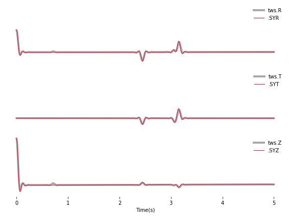
We see that the Waveforms of Pyraysum (red) and Teleweavesim (gray)
match pretty well. The Telewavsim data has some additional energy at
about 0.9 seconds, which is a reflection from the top of the anisotropic
layer. This reflections has explicitly not been computed
(RC.mults = 0), but this could be done using RC.set_phaselist().
Conclusion
In this example we have explored the capabilities of Pyraysum to compute synthetic seismograms and receiver functions for dipping or anisotropic layers. We have compared the outcome of our simulations with published results and, for the anisotropic example, also with synthetic data from another numerical method. Both comparisons showed that Pyraysum delivers comparable results.
References
Audet, P., Thomson, C.J., Bostock, M.G., and Eulenfeld, T. (2019). Telewavesim: Python software for teleseismic body wave modeling. Journal of Open Source Software, 4(44), 1818, https://doi.org/10.21105/joss.01818
Porter, R., Zandt, G., & McQuarrie, N. (2011). Pervasive lower-crustal seismic anisotropy in Southern California: Evidence for underplated schists and active tectonics. Lithosphere, 3(3), 201-220. https://doi.org/10.1130/L126.1
Thomson, C.J. (1997). Modelling surface waves in anisotropic structures: I. Theory. Physics of the Earth and Planetary interiors, 103, 195-206. https://doi.org/10.1016/S0031-9201(97)00033-2