Tutorials
Creating the StDb Database
All the scripts provided require a StDb database containing station
information and metadata. Let’s first create this database for station
TGTN and send the prompt to a logfile
$ query_fdsn_stdb -N NY -C HH -S TGTN TGTN > logfile
To check the station info for TGTN, use the program ls_stdb:
$ ls_stdb TGTN.pkl
Listing Station Pickle: TGTN.pkl
NY.TGTN
--------------------------------------------------------------------------
1) NY.TGTN
     Station: NY TGTN
      Alternate Networks: None
      Channel: HH ;  Location: --
      Lon, Lat, Elev:  61.52670, -128.27269,   0.000
      StartTime: 2013-07-01 00:00:00
      EndTime:   2020-05-20 13:34:38
      Status:    partial
      Polarity: 1
      Azimuth Correction: 0.000000
Automated analysis
There are two modes for producing shear-wave splitting estimates: Automated or Manual. In the automated mode, the code uses default uniform settings for all available seismograms to produce splitting estimates. In the manual mode, the code will search for available (pre-processed) data on disk and use a Graphical-User Interface (GUI) to refine the analysis window based on new picks. If the automated estimates are not available, they will first be determined before refining the window.
Downloading data
Simply run split_calc_auto with TGTN.pkl to download all available
seismic data suitable for shear-wave splitting analysis.
$ split_calc_auto --keys=NY.TGTN --start=2020-01-01 --end=2020-05-20 TGTN.pkl
This uses all default settings for window lengths, magnitude criteria, etc.
In this example, the program will search on the specific data server
(through obspy clients) to download the waveforms. Here, only events that occurred between January 1, 2020 and May 20, 2020 will
be considered. Based on the criteria specified (see split_calc_auto), seismograms will be
downloaded where the minimum SNR threshold is exceeded. All data will be saved in separate
time-key folders to PATH/NY.TGTN/YYYYMMDD_HRMNSC/*.
Downloading and Processing
You can run split_calc_auto to automatically estimate the shear-wave splitting
parameters by specifying the argument or --calc. Choosing -V
or --verbose will display
the results to the terminal as the script proceeds. If you wish to visualize the results
for each event, you can further select --plot-diagnostic. This will pop a
summary Figure (i.e., Figure 1) of the splitting results for this particular event.
As an example of a Good, non-null estimate, type the following line in the terminal
(note the argument -O to overwrite existing results, and no key is specified since
there is only one key in the database):
$ split_calc_auto --start=2020-03-18 --end=2020-03-19 -V --calc --plot-diagnostic -O TGTN.pkl
This will produce, in the terminal:
###################################################################
#            _ _ _                _                     _         #
#  ___ _ __ | (_) |_     ___ __ _| | ___     __ _ _   _| |_ ___   #
# / __| '_ \| | | __|   / __/ _` | |/ __|   / _` | | | | __/ _ \  #
# \__ \ |_) | | | |_   | (_| (_| | | (__   | (_| | |_| | || (_) | #
# |___/ .__/|_|_|\__|___\___\__,_|_|\___|___\__,_|\__,_|\__\___/  #
#     |_|          |_____|             |_____|                    #
#                                                                 #
###################################################################

|==================================================|
|                       TGTN                       |
|==================================================|
|  Station: NY.TGTN                                |
|      Channel: HH; Locations: --                  |
|      Lon: -128.27; Lat:  61.53                   |
|      Start time: 2013-07-01 00:00:00             |
|      End time:   2020-05-20 13:34:38             |
|--------------------------------------------------|
| Searching Possible events:                       |
|   Start: 2020-03-18 00:00:00                     |
|   End:   2020-03-19 00:00:00                     |
|   Mag:   >{0:3.1f} 6.0                           |
| ...                                              |
|  Found     2 possible events                     |
|==================================================|

**************************************************
* #1 (2/2):  20200318_031345 NY.TGTN
*   Phase: SKS
*   Origin Time: 2020-03-18 03:13:45
*   Lat: -13.14;        Lon:  167.03
*   Dep: 176.00 km;     Mag: 6.1
*   Dist: 10000.87 km;   Epi dist:  89.94 deg
*   Baz:  241.82 deg;   Az:  25.63 deg
* Requesting Waveforms:
*    Startime: 2020-03-18 03:34:38
*    Endtime:  2020-03-18 03:38:38
*     TGTN.HH - ZNE:
*          HH[ZNE].-- - Checking Network
*              - ZNE Data Downloaded
* Start times are not all close to true start:
*   HHE 2020-03-18T03:34:38.110000Z 2020-03-18T03:38:39.100000Z
*   HHN 2020-03-18T03:34:38.110000Z 2020-03-18T03:38:39.100000Z
*   HHZ 2020-03-18T03:34:38.110000Z 2020-03-18T03:38:39.100000Z
*   True start: 2020-03-18T03:34:38.107273Z
* -> Shifting traces to true start
* Waveforms Retrieved...
* SNRQ: 12.51340359244245
* SNRT: 8.8889144288134
* --> Calculating Rotation-Correlation (RC) Splitting
* --> Calculating Silver-Chan (SC) Splitting
*     Null Classification:
*       SNR T Pass: 8.89 > 1.00
*       dPhi Pass:  3.00 outside 22. < X < 68.
*     Quality Estimate: Non-Null -- Good
*         rho: 1.00; dphi: 3.00
*           Good: 0.8 < rho < 1.1  &&  dphi < 8
*           Fair: 0.7 < rho < 1.2  &&  dphi < 15
*           Poor: rho < 0.7 | rho > 1.3 &&  dphi > 15
 ======= Meta data ========

 SNR (dB):            13
 Station:             TGTN
 Time:                2020-03-18T03:13:45.742000Z
 Event depth (km):    0
 Magnitude (Mw):      6.1
 Longitude (deg):     167.03
 Latitude (deg):      -13.14
 GAC (deg):           89.94
 Backazimuth deg):    241.82
 Incidence (deg):      10.17
 SNR - Q:      12.51
 SNR - T:      8.89

 ======= Best-fit splitting results ========

 Best fit values: RC method
 Phi = -75 degrees +/-  7
 dt = 1.3 seconds +/- 0.1

 Best fit values: SC method
 Phi = -78 degrees +/-  5
 dt = 1.3 seconds +/- 0.2

 ======= Nulls and quality ========

 Is Null?      False
 Quality:      Good
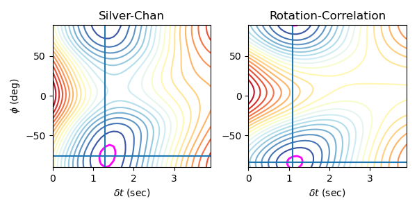
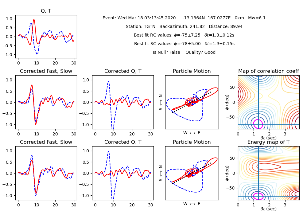
Figure 1 summarizes the results of the splitting calculation. The top left “Q,T”
frame shows the un-corrected radial (Q) and tangential (T) components within the
time window. The second row of panels correspond to the ‘Rotation-Correlation’
results, and the third row of panels is for the ‘Silver-Chan’ results. In each
case, the first column shows the corrected Q and T fast and slow components, the
second column the corrected Q and T components, the third column the before and after
particle motion, and the fourth column the map of the error surfaces. A text box
prints out the summary of the results, including whether or not the estimate is a
Null, and the quality of the estimate (‘good’, ‘fair’, ‘poor’).
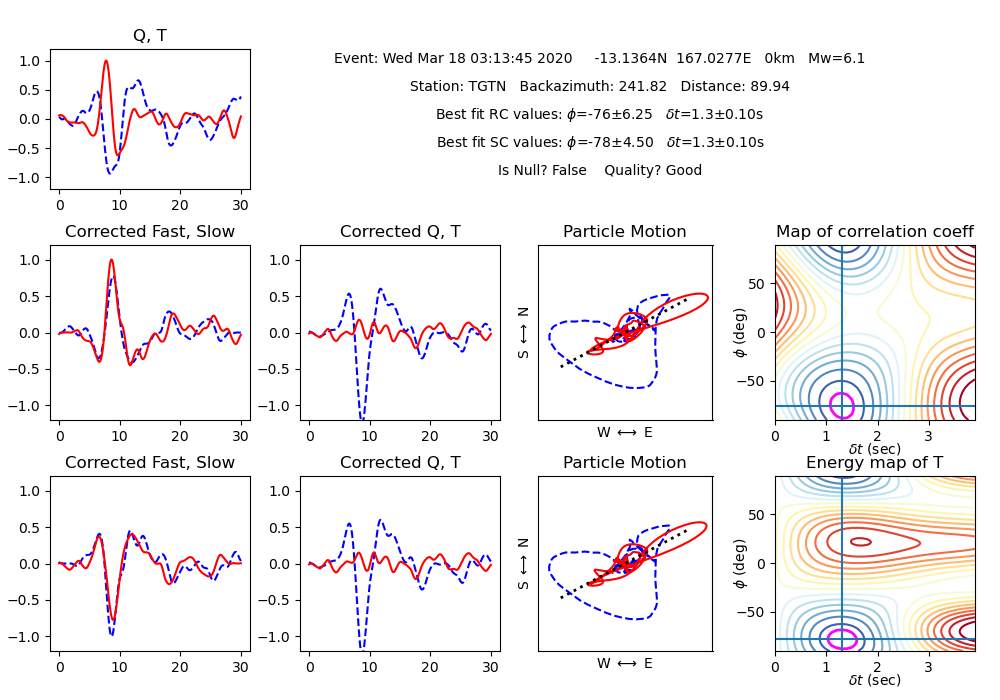
Re-Processing
It is also possible to re-calculate the estimates for different parameters using the
argument --recalc, which will be applied uniformly to all available data.
In this case the data will not be re-downloaded and the data files will simply be updated
in place. Plotting can also be done as in the previous example. For example, let’s
change the frequency settings and re-calculate the previous example:
$ split_calc_auto --start=2020-03-18 --end=2020-03-19 --fmin=0.05 --fmax=1. -V --recalc --plot-diagnostic -O TGTN.pkl
This will produce, in the terminal:
###################################################################
#            _ _ _                _                     _         #
#  ___ _ __ | (_) |_     ___ __ _| | ___     __ _ _   _| |_ ___   #
# / __| '_ \| | | __|   / __/ _` | |/ __|   / _` | | | | __/ _ \  #
# \__ \ |_) | | | |_   | (_| (_| | | (__   | (_| | |_| | || (_) | #
# |___/ .__/|_|_|\__|___\___\__,_|_|\___|___\__,_|\__,_|\__\___/  #
#     |_|          |_____|             |_____|                    #
#                                                                 #
###################################################################

|==================================================|
|                       TGTN                       |
|==================================================|
|  Station: NY.TGTN                                |
|      Channel: HH; Locations: --                  |
|      Lon: -128.27; Lat:  61.53                   |
|      Start time: 2013-07-01 00:00:00             |
|      End time:   2020-05-20 13:34:38             |
|--------------------------------------------------|
| Searching Possible events:                       |
|   Start: 2020-03-18 00:00:00                     |
|   End:   2020-03-19 00:00:00                     |
|   Mag:   >{0:3.1f} 6.0                           |
| ...                                              |
|  Found     2 possible events                     |
|==================================================|

**************************************************
* #1 (2/2):  20200318_031345 NY.TGTN
*   Phase: SKS
*   Origin Time: 2020-03-18 03:13:45
*   Lat: -13.14;        Lon:  167.03
*   Dep: 176.00 km;     Mag: 6.1
*   Dist: 10000.87 km;   Epi dist:  89.94 deg
*   Baz:  241.82 deg;   Az:  25.63 deg
* SNRQ: 13.03806173520674
* SNRT: 8.36765404740968
* --> Calculating Rotation-Correlation (RC) Splitting
* --> Calculating Silver-Chan (SC) Splitting
*     Null Classification:
*       SNR T Pass: 8.37 > 1.00
*       dPhi Pass:  2.00 outside 22. < X < 68.
*     Quality Estimate: Non-Null -- Good
*         rho: 1.00; dphi: 2.00
*           Good: 0.8 < rho < 1.1  &&  dphi < 8
*           Fair: 0.7 < rho < 1.2  &&  dphi < 15
*           Poor: rho < 0.7 | rho > 1.3 &&  dphi > 15
 ======= Meta data ========

 SNR (dB):            13
 Station:             TGTN
 Time:                2020-03-18T03:13:45.742000Z
 Event depth (km):    0
 Magnitude (Mw):      6.1
 Longitude (deg):     167.03
 Latitude (deg):      -13.14
 GAC (deg):           89.94
 Backazimuth deg):    241.82
 Incidence (deg):      10.17
 SNR - Q:      13.04
 SNR - T:      8.37

 ======= Best-fit splitting results ========

 Best fit values: RC method
 Phi = -76 degrees +/-  6
 dt = 1.3 seconds +/- 0.1

 Best fit values: SC method
 Phi = -78 degrees +/-  4
 dt = 1.3 seconds +/- 0.1

 ======= Nulls and quality ========

 Is Null?      False
 Quality:      Good
Manual analysis
In the manual mode, the script split_calc_manual will use the available data and/or estimates and use a Graphical User Interface (GUI) to refine the picking window. The script will search for data and splitting estimates in the folder structure. If the estimates are not available (i.e., not previously calculated in split_calc_auto), the script will calculate them automatically.
Re-picking
After loading/processing the automated results, the script will produce two Figures.
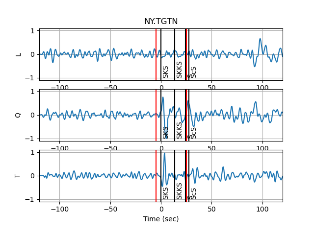
Figure 1 shows the three
rotated component waveforms (LQT), along with lines representing the SKS, SKKS,
S, PKS and ScS arrivals from model iasp91. Red vertical lines denote the analysis
window. This figure is interactive and the picks in red can be refined by clicking
at the two x-positions of the new analysis window.
From the previous example, examining and possibly refining the results for only one day of data:
$ split_calc_manual --start=2020-03-18 --end=2020-03-19 TGTN.pkl
The diagnostic (summary) figure (Figure 2) will also open, showing the results
from the most recent automated estimate (i.e., can be from a re-calculated estimate,
see split_calc_auto). A message box will pop up asking whether to Re-pick the
window in Figure 1. This is done to refine the signal window in
which the measurements are made in order to eliminate possibly contaminating phases
and improve the measurements. If the -V or --verbose argument has been
selected, the terminal will show a summary of the processing, as in previous examples.
Once No is selected for the picking/re-picking of the window, a second box
will pop up asking whether to keep the estimates. Click Yes to save the results,
or No to discard the measurement.
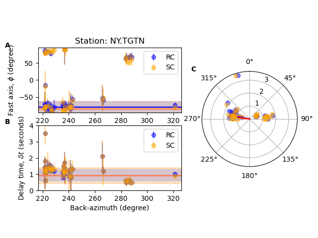
Station average
Plotting and subsequent processing of splitting results is carried out using
split_average, where options are present to control selection of nulls
and quality settings, as well as which methods are used. All available data are
processed. By default, the script will search for the manual results. The user
can specify to use the auto results with the argument --auto. The final
average splits are then saved in a text file for future use.
For example, after running the refined processing for 4 years of data for station
TGTN (i.e., typing split_calc_auto --start=2016-01-01 --end=2020-06-01 -V --calc TGTN.pkl, which will
take a long time to run and process all the data), we can visualize the results
by typing in a terminal:
$ split_average --show-fig -V --auto TGTN.pkl

###############################################################
#            _ _ _                                            #
#  ___ _ __ | (_) |_     __ ___   _____ _ __ __ _  __ _  ___  #
# / __| '_ \| | | __|   / _` \ \ / / _ \ '__/ _` |/ _` |/ _ \ #
# \__ \ |_) | | | |_   | (_| |\ V /  __/ | | (_| | (_| |  __/ #
# |___/ .__/|_|_|\__|___\__,_| \_/ \___|_|  \__,_|\__, |\___| #
#     |_|          |_____|                        |___/       #
#                                                             #
###############################################################

---------------------------
Selection Criteria
 Null Value:
    Non Nulls: True
    Nulls:     False
 Quality Value:
    Goods:  True
    Fairs:  True
    Poors:  False
---------------------------
  Found 136 event folders...
  Checking 'auto' results...
      20160302_124948 Poor Null -> Skipped
      20160401_192455 Good Non-Null -> Retained
      20160403_082352 Poor Non-Null -> Skipped
      20160406_065848 Poor Null -> Skipped
      20160407_033253 Good Non-Null -> Retained
      20160413_135517 Fair Non-Null -> Retained
      20160414_215027 Poor Null -> Skipped
      20160428_193324 Poor Non-Null -> Skipped
      20160527_040843 Good Non-Null -> Retained
      ...

*** Estimates from averaging 41 error surfaces ***
   PHI (RC):   -84.0 d +/- 3.75
   DT (RC):      1.1 s +/- 0.08
   PHI (SC):   -76.0 d +/- 6.75
   DT (SC):      1.3 s +/- 0.07
   PHI (mean):   -80.0 d +/- 5.25
   DT (mean):      1.2 s +/- 0.07
   Saved to:
      RESULTS/NY.TGTN_Nons_G-F_RC_ES_average.dat
      RESULTS/NY.TGTN_Nons_G-F_SC_ES_average.dat
2025-05-19 16:14:07.247 python3.12[48658:4945516] The class 'NSSavePanel' overrides the method identifier.  This method is implemented by class 'NSWindow'

*** Estimates from averaging 41 individual measurements ***
   PHI (RC):   -79.1 d +/- 17.16
   DT (RC):      0.9 s +/- 0.38
   PHI (SC):   -84.4 d +/- 21.77
   DT (SC):      0.9 s +/- 0.52
   PHI (mean): -81.8 d +/- 19.5
   DT (mean):    0.9 s +/- 0.5
   Saved to:
      RESULTS/NY.TGTN_Nons_G-F_RC_ind_average.dat
      RESULTS/NY.TGTN_Nons_G-F_SC_ind_average.dat

*** Catalogue of events and individual results ***
   Saved to:
      RESULTS/NY.TGTN_Nons_G-F_events.dat