Telewavesim is a software for modeling teleseismic (i.e., planar) body wave propagation through stacks of anisotropic layers for receiver based studies.

Licence¶

Permission is hereby granted, free of charge, to any person obtaining a copy of this software and associated documentation files (the “Software”), to deal in the Software without restriction, including without limitation the rights to use, copy, modify, merge, publish, distribute, sublicense, and/or sell copies of the Software, and to permit persons to whom the Software is furnished to do so, subject to the following conditions:

The above copyright notice and this permission notice shall be included in all copies or substantial portions of the Software.

THE SOFTWARE IS PROVIDED “AS IS”, WITHOUT WARRANTY OF ANY KIND, EXPRESS OR IMPLIED, INCLUDING BUT NOT LIMITED TO THE WARRANTIES OF MERCHANTABILITY, FITNESS FOR A PARTICULAR PURPOSE AND NONINFRINGEMENT. IN NO EVENT SHALL THE AUTHORS OR COPYRIGHT HOLDERS BE LIABLE FOR ANY CLAIM, DAMAGES OR OTHER LIABILITY, WHETHER IN AN ACTION OF CONTRACT, TORT OR OTHERWISE, ARISING FROM, OUT OF OR IN CONNECTION WITH THE SOFTWARE OR THE USE OR OTHER DEALINGS IN THE SOFTWARE.

Installation¶

Dependencies¶

The current version works well with Python>3.5. Also, the following packages are required:

gfortran (or any Fortran compiler)
obspy

By default, both numpy and matplotlib are installed as dependencies of obspy.

Conda environment¶

We recommend creating a custom conda environment where telewavesim can be installed along with its dependencies:

conda create -n tws python=3.7 obspy -c conda-forge

Activate the newly created environment:

conda activate tws

Installing latest version from PyPi¶

Install the latest version from PyPi with the following command:

pip install telewavesim

Installing development version from source¶

Clone the repository:

git clone https://github.com/paudetseis/Telewavesim.git
cd Telewavesim

Install using pip:

pip install .

Possible installation pitfalls with conda¶

Using conda it might be necessary to use the fortran compiler provided with conda-forge. Add fortran-compiler package to the above conda environment calls. On Linux it might further be necessary to install the lapack conda package.

Testing¶

A series of tests are located in the tests subdirectory. In order to perform these tests, run pytest (conda install pytest if needed):

pytest -v --pyargs telewavesim

Usage¶

Jupyter Notebooks¶

Included in this package is a set of Jupyter Notebooks (see Table of Content), which give examples on how to call the various routines and obtain plane wave seismograms and receiver functions. The Notebooks describe how to reproduce published examples of synthetic data from Audet (2016) and Porter et al. (2011).

After telewaveim, these notebooks can be locally installed (i.e., in a local folder Notebooks) from the package by typing in a python window:

from telewavesim import doc
doc.install_doc(path='Notebooks')

To run the notebooks you will have to further install jupyter. From the terminal, type:

conda install jupyter

Followed by:

cd Notebooks
jupyter notebook

You can then save the notebooks as python scripts, check out the model files and set up your own examples.

Setting up new models¶

From the model file¶

In the Jupiter notebooks you will find a folder named models where a few examples are provided. The header of the file model_Audet2016.txt looks like:

################################################
#
#   Model file to use with `telewavesim` for
#   modeling teleseismic body wave propagation
#   through stratified media.
#
#   Lines starting with '#' are ignored. Each
#   line corresponds to a unique layer. The
#   bottom layer is assumed to be a half-space
#   (Thickness is irrelevant).
#
#   Format:
#       Column  Contents
#          0    Thickness (km)
#          1    Density (kg/m^3)
#          2    Layer P-wave velocity (km/s)
#          3    Layer S-wave velocity (km/s)
#          4    Layer flag
#                   iso: isotropic
#                   tri: transverse isotropy
#                   [other]: other minerals or rocks
#          5    % Transverse anisotropy (if Layer is set to 'tri')
#                   0: isotropic
#                   +: fast symmetry axis
#                   -: slow symmetry axis
#          6    Trend of symmetry axis (degrees)
#          7    Plunge of symmetry axis (degrees)
#
################################################

The header is not required and can be deleted when you become familiar with the various definitions. Note that the code requires 8 entries per layer, regardless of whether or not the variable is required (it will simply be ignored if it’s not).

Let us break down each line, depending on how you set Layer flag:

Layer flag set to `iso`¶

This flag represents a case where the layer is isotropic.

Set column 0 (Thickness), column 1 (Density), column 2 (P-wave velocity), column 3 (S-wave velocity) and column 4 (as iso)
Set columns 5 to 7 to 0. or any other numerical value - they will be ignored by the software.

Layer flag set to `tri`¶

This flag represents a transversely isotropic layer. We adhere with the definition in Porter et al. (2011), whereby the parameter \(\eta\), which describes the curvature of the velocity “ellipsoid” between the \(V_P\)-fast and \(V_P\)-slow axes, varies with anisotropy for a 2-\(\psi\) model and is not fixed.

The column 5 in this case sets the percent anisotropy for both \(V_P\) and \(V_S\) (equal anisotropy for both \(V_P\) and \(V_S\)) and is the only instance where this column is required.

Set all columns to the required numerical value (and column 4 to tri)

Layer flag set to another type of material¶

This flag should be set to the specific single-crystal or rock abbreviation, for which the elastic properties have been determined in the lab. Currently available options are:

mins = ['atg', 'bt', 'cpx', 'dol', 'ep', 'grt', 'gln', 'hbl', 'jade', 'lws', 'lz', 'ms', 'ol', 'opx', 'plag', 'qtz', 'zo']

rocks = ['BS_f', 'BS_m', 'EC_f', 'EC_m', 'HB', 'LHZ', 'SP_37', 'SP_80']

The module elast contains the definition of the stiffness matrices for these minerals and rocks. Check out the module or the documentation for more details.

Set entries in column 0 (Thickness), column 4 (an abbreviation among the above options), and optionally columns 6 and 7 if you wish to rotate the corresponding tensor about two axes (trend and plunge of the equivalent of the symmetry axis in transverse isotropy). Columns 1 to 3 can be set to any numerical value and will be ignored by the software.

Note

The code can handle general anisotropy (with 21 independent components in the elastic tensor) for any type of material. Currently, however, the code contains a limited number of elastic tensors (see elast) but we encourage users to suggest their own tensors determined from the lab. This can be done by raising an issue on the GitHub page or making a pull request with the suggested addition to the elast module.

From the Model class¶

Models can also be defined on the fly in Python using lists that contain the relevant information as input into an instance of the Model class.

Examples

>>> from telewavesim.utils import Model

Define a two-layer model with isotropic properties

>>> thick = [20., 0]       # Second layer thickness is irrelevant
>>> rho = [2800., 3300.]   # Second rho value is irrelevant as we use a pre-defined elastic tensor
>>> vp = [4.6, 6.]         # Likewise for vp
>>> vs = [2.6, 3.6]        # Likewise for vs
>>> flag = ['iso', 'iso']  # Both layers are isotropic
>>> model = Model(thick, rho, vp, vs, flag)

Define a two-layer model with foliated eclogitic crust over isotropic half-space

>>> # Example using a single line
>>> model = Model([20, 0], [None, 3300.], [0, 6.0], [0, 3.6], ['EC_f', 'iso'], [0, 0], [0, 0], [0, 0])

Note

In this example we did not specify the last 3 entries (% aniso, trend, plunge), such that the tensor is aligned with a horizontal axis (plunge of 0) of symmetry pointing North (trend of 0).

Define a two-layer model with transversely isotropic crust over isotropic half-space

>>> # Example using a single line
>>> model = Model([20., 0.], [2800., 3300.], [4., 6.], [2.6, 3.6], ['tri', 'iso'], [5., 0], [30., 0], [10., 0])

Note

In this example all entries for the first layer are required. Here the anisotropy is set to 5% (i.e., fast axis of symmetry; for slow axis the user should input -5.) and the axis of symmetry has a trend of 30 degrees and a plunge of 10 degrees.

Define a three-layer model with isotropic crust and antigorite upper mantle layer over isotropic half-space

>>> thick = [20., 10., 0]        # Third layer thickness is irrelevant
>>> rho = [2800., None, 3300.]   # Second rho value is irrelevant as we use a pre-defined elastic tensor
>>> vp = [4.6, 0., 6.]           # Likewise for vp
>>> vs = [2.6, 0., 3.6]          # Likewise for vs
>>> flag = ['iso', 'atg', 'iso'] # Specifies the second layer as 'antigorite'
>>> pct_aniso = [None, None, None]     # Percent anisotropy - irrelevant as we use a pre-defined elastic tensor
>>> trend = [0., 45., 0.]        # Trend of 45 degrees for the antigorite layer
>>> plunge = [0., 20., 0.]       # Plunge of 20 degrees for the antigorite layer
>>> model = Model(thick, rho, vp, vs, flag, pct_aniso, trend, plunge)
>>> model.rho
array([2800.0, 2620.0, 3300.0], dtype=object)
>>> model.isoflg
['iso', 'atg', 'iso']

Basic usage¶

These examples are extracted from the run_plane() function.

By default, the function uses a back-azimuth value of 0 degree, which is suitable for events coming from the North pole or isotropic seismic velocity models (i.e., those that do not vary with direction of incoming waves).

For anisotropic velocity models, users need to specify the back-azimuth value in degrees. Furthermore, the default type of the incoming teleseismic body wave is 'P' for compressional wave. Other options are 'SV', 'SH', or 'Si' for vertically-polarized shear wave, horizontally-polarized shear wave or isotropic shear wave, respectively. Wave modes cannot be mixed.

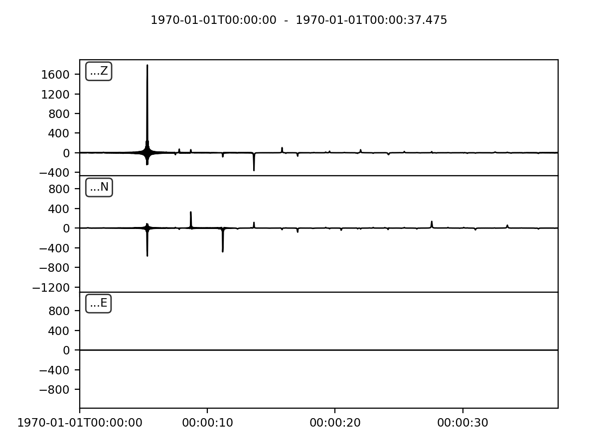
Modeling a single event¶

>>> from telewavesim import utils
>>> # Define three-layer model with isotropic crust and antigorite upper mantle layer over isotropic half-space
>>> model = utils.Model([20, 10, 0], [2800., None, 3300.], [4.6, 0, 6.0], [2.6, 0, 3.6], ['iso', 'atg', 'iso'], [0, 0, 0], [0, 0, 0], [0, 0, 0])
>>> slow = 0.06     # s/km
>>> npts = 1500
>>> dt = 0.025      # s
>>> st = utils.run_plane(model, slow, npts, dt)

>>> type(st)
<class 'obspy.core.stream.Stream'>
>>> print(st)
3 Trace(s) in Stream:
...N | 1970-01-01T00:00:00.000000Z - 1970-01-01T00:00:37.475000Z | 40.0 Hz, 1500 samples
...E | 1970-01-01T00:00:00.000000Z - 1970-01-01T00:00:37.475000Z | 40.0 Hz, 1500 samples
...Z | 1970-01-01T00:00:00.000000Z - 1970-01-01T00:00:37.475000Z | 40.0 Hz, 1500 samples
>>> st.plot(size=(600, 450))

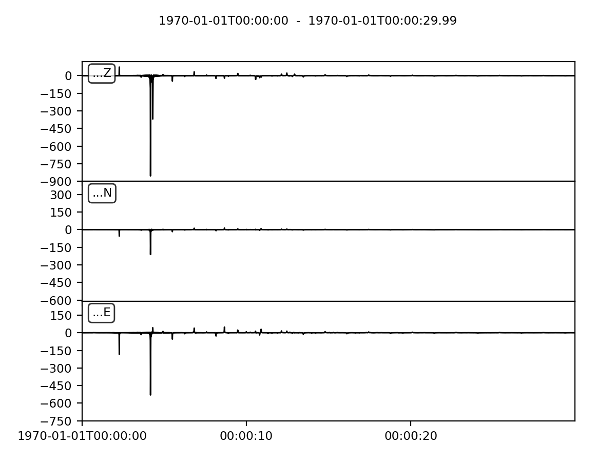
Single event for OBS station¶

>>> from telewavesim import utils
>>> # Define two-layer model with foliated eclogitic crust over isotropic half-space
>>> model = utils.Model([20, 0], [None, 3300.], [0, 6.0], [0, 3.6], ['EC_f', 'iso'], [0, 0], [0, 0], [0, 0])
>>> slow = 0.06     # s/km
>>> npts = 3000
>>> dt = 0.01      # s
>>> wvtype = 'SV'
>>> baz = 45.
>>> dp = 1000.
>>> st = utils.run_plane(model, slow, npts, dt, baz=baz, wvtype=wvtype, obs=True, dp=dp)
>>> st.plot(size=(600, 450))

Licence¶

Installation¶

Dependencies¶

Conda environment¶

Installing latest version from PyPi¶

Installing development version from source¶

Possible installation pitfalls with conda¶

Testing¶

Usage¶

Jupyter Notebooks¶

Setting up new models¶

From the model file¶

Layer flag set to iso¶

Layer flag set to tri¶

Layer flag set to another type of material¶

From the Model class¶

Basic usage¶

Modeling a single event¶

Single event for OBS station¶

Layer flag set to `iso`¶

Layer flag set to `tri`¶